• Chi-Square Independence Test - What Is It?
• Null Hypothesis
• Assumptions
• Test Statistic
• Effect Size
• Reporting

Chi-Square Independence Test - What Is It?

The chi-square independence test evaluates if
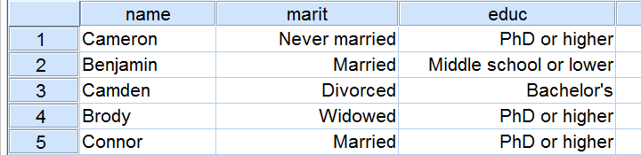
two categorical variables are related in some population. Example: a scientist wants to know if education level and marital status are related for all people in some country. He collects data on a simple random sample of n = 300 people, part of which are shown below.

Chi-Square Test - Observed Frequencies

A good first step for these data is inspecting the contingency table of marital status by education. Such a table -shown below- displays the frequency distribution of marital status for each education category separately. So let's take a look at it.

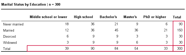
The numbers in this table are known as the observed frequencies. They tell us an awful lot about our data. For instance,

• there's 4 marital status categories and 5 education levels;
• we succeeded in collecting data on our entire sample of n = 300 respondents (bottom right cell);
• we've 84 respondents with a Bachelor’s degree (bottom row, middle);
• we've 30 divorced respondents (last column, middle);
• we've 9 divorced respondents with a Bachelor’s degree.

Chi-Square Test - Column Percentages

Although our contingency table is a great starting point, it doesn't really show us if education level and marital status are related. This question is answered more easily from a slightly different table as shown below.

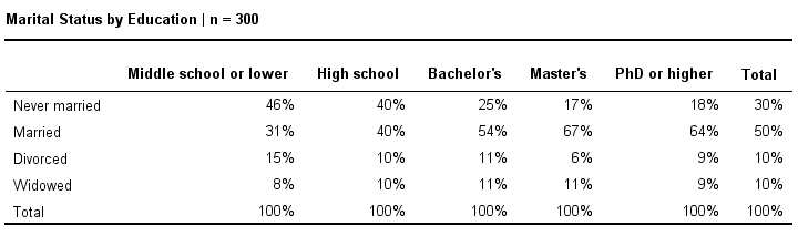
This table shows -for each education level separately- the percentages of respondents that fall into each marital status category. Before reading on, take a careful look at this table and tell me is marital status related to education level and -if so- how? If we inspect the first row, we see that 46% of respondents with middle school never married. If we move rightwards (towards higher education levels), we see this percentage decrease: only 18% of respondents with a PhD degree never married (top right cell).

Reversely, note that 64% of PhD respondents are married (second row). If we move towards the lower education levels (leftwards), we see this percentage decrease to 31% for respondents having just middle school. In short, more highly educated respondents marry more often than less educated respondents.

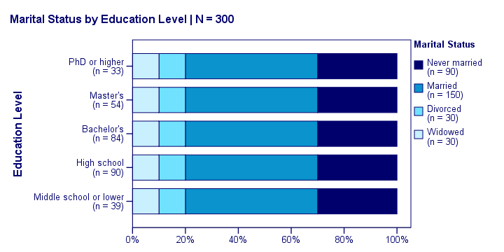
Chi-Square Test - Stacked Bar Chart

Our last table shows a relation between marital status and education. This becomes much clearer by visualizing this table as a stacked bar chart, shown below.

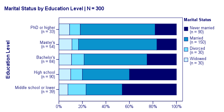
If we move from top to bottom (highest to lowest education) in this chart, we see the dark blue bar (never married) increase. Marital status is clearly associated with education level.The lower someone’s education, the smaller the chance he’s married. That is: education “says something” about marital status (and reversely) in our sample. So what about the population?

Chi-Square Test - Null Hypothesis

The null hypothesis for a chi-square independence test is that two categorical variables are independent in some population. Now, marital status and education are related -thus not independent- in our sample. However, we can't conclude that this holds for our entire population. The basic problem is that samples usually differ from populations.

If marital status and education are perfectly independent in our population, we may still see some relation in our sample by mere chance. However, a strong relation in a large sample is extremely unlikely and hence refutes our null hypothesis. In this case we'll conclude that the variables were not independent in our population after all.

So exactly how strong is this dependence -or association- in our sample? And what's the probability -or p-value- of finding it if the variables are (perfectly) independent in the entire population?

Chi-Square Test - Statistical Independence

Before we continue, let's first make sure we understand what “independence” really means in the first place. In short, independence means that one variable doesn't
“say anything” about another variable. A different way of saying the exact same thing is that independence means that the relative frequencies of one variable
are identical over all levels of some other variable. Uh... say again? Well, what if we had found the chart below?

What does education “say about” marital status? Absolutely nothing! Why? Because the frequency distributions of marital status are identical over education levels: no matter the education level, the probability of being married is 50% and the probability of never being married is 30%.

In this chart, education and marital status are perfectly independent. The hypothesis of independence tells us which frequencies we should have found in our sample: the expected frequencies.

Expected Frequencies

Expected frequencies are the frequencies we expect in a sample
if the null hypothesis holds. If education and marital status are independent in our population, then we expect this in our sample too. This implies the contingency table -holding expected frequencies- shown below.

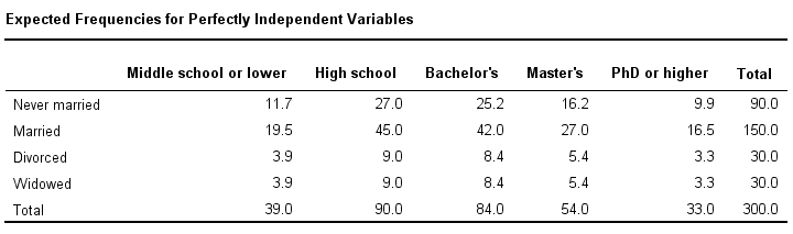
These expected frequencies are calculated as $$eij = \frac{oi\cdot oj}{N}$$
where

• \(eij\) is an expected frequency;
• \(oi\) is a marginal column frequency;
• \(oj\) is a marginal row frequency;
• \(N\) is the total sample size.

So for our first cell, that'll be $$eij = \frac{39 \cdot 90}{300} = 11.7$$
and so on. But let's not bother too much as our software will take care of all this.

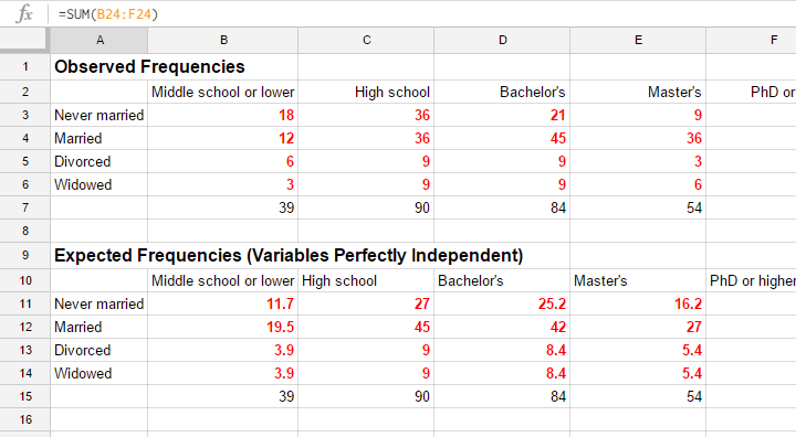
Note that many expected frequencies are non integers. For instance, 11.7 respondents with middle school who never married. Although there's no such thing as “11.7 respondents” in the real world, such non integer frequencies are just fine mathematically. So at this point, we've 2 contingency tables:

• a contingency table with observed frequencies we found in our sample;
• a contingency table with expected frequencies we should have found in our sample if the variables are really independent.

The screenshot below shows both tables in this GoogleSheet (read-only). This sheet demonstrates all formulas that are used for this test.

Residuals

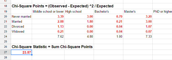
Insofar as the observed and expected frequencies differ, our data deviate more from independence. So how much do they differ? First off, we subtract each expected frequency from each observed frequency, resulting in a residual. That is, $$rij = oij - eij$$
For our example, this results in (5 * 4 =) 20 residuals. Larger (absolute) residuals indicate a larger difference between our data and the null hypothesis. We basically add up all residuals, resulting in a single number: the χ² (pronounce “chi-square”) test statistic.

Test Statistic

The chi-square test statistic is calculated as
$$\chi^2 = \Sigma{\frac{(oij - eij)^2}{eij}}$$
so for our data $$\chi^2 = \frac{(18 - 11.7)^2}{11.7} + \frac{(36 - 27)^2}{27} + ... + \frac{(6 - 5.4)^2}{5.4} = 23.57$$

Again, our software will take care of all this. But if you'd like to see the calculations, take a look at this GoogleSheet.

So χ² = 23.57 in our sample. This number summarizes the difference between our data and our independence hypothesis. Is 23.57 a large value? What's the probability of finding this? Well, we can calculate it from its sampling distribution but this requires a couple of assumptions.

Chi-Square Test Assumptions

The assumptions for a chi-square independence test are

1. independent observations. This usually -not always- holds if each case in SPSS holds a unique person or other statistical unit. Since this is the case for our data, we'll assume this has been met.
2. For a 2 by 2 table, all expected frequencies > 5.However, for a 2 by 2 table, a z-test for 2 independent proportions is preferred over the chi-square test.
   
   For a larger table, all expected frequencies > 1 and no more than 20% of all cells may have expected frequencies < 5.

If these assumptions hold, our χ² test statistic follows a χ² distribution. It's this distribution that tells us the probability of finding χ² > 23.57.

Chi-Square Test - Degrees of Freedom

We'll get the p-value we're after from the chi-square distribution if we give it 2 numbers:

• the χ² value (23.57) and
• the degrees of freedom (df).

The degrees of freedom is basically a number that determines the exact shape of our distribution. The figure below illustrates this point.

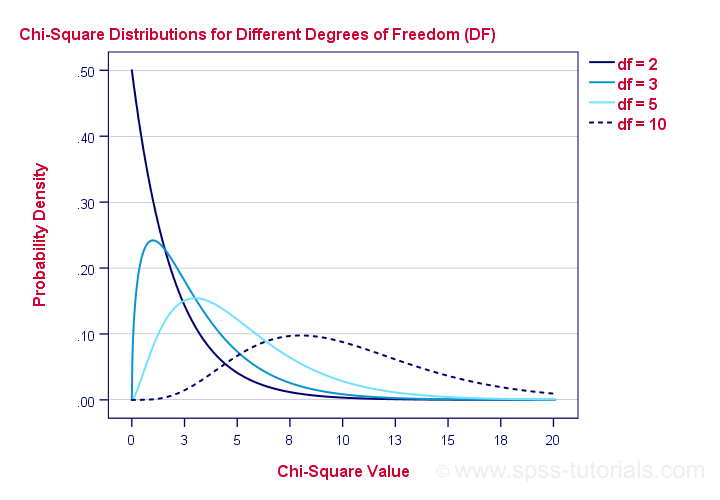
Right. Now, degrees of freedom -or df- are calculated as $$df = (i - 1) \cdot (j - 1)$$
where

• \(i\) is the number of rows in our contingency table and
• \(j\) is the number of columns

so in our example $$df = (5 - 1) \cdot (4 - 1) = 12.$$
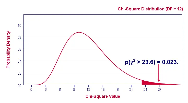
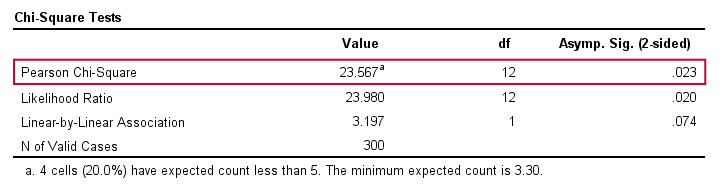
And with df = 12, the probability of finding χ² ≥ 23.57 ≈ 0.023.We simply look this up in SPSS or other appropriate software. This is our 1-tailed significance. It basically means, there's a 0.023 (or 2.3%) chance of finding this association in our sample if it is zero in our population.

Since this is a small chance, we no longer believe our null hypothesis of our variables being independent in our population. Conclusion: marital status and education are related
in our population. Now, keep in mind that our p-value of 0.023 only tells us that the association between our variables is probably not zero. It doesn't say anything about the strength of this association: the effect size.

Effect Size

For the effect size of a chi-square independence test, consult the appropriate association measure. If at least one nominal variable is involved, that'll usually be Cramér’s V (a sort of Pearson correlation for categorical variables). In our example Cramér’s V = 0.162. Since Cramér’s V takes on values between 0 and 1, 0.162 indicates a very weak association. If both variables had been ordinal, Kendall’s tau or a Spearman correlation would have been suitable as well.

Reporting

For reporting our results in APA style, we may write something like “An association between education and marital status was observed, χ²(12) = 23.57, p = 0.023.”

Chi-Square Independence Test - Software

You can run a chi-square independence test in Excel or Google Sheets but you probably want to use a more user friendly package such as

• SPSS,
• Stata or
• SAS.

The figure below shows the output for our example generated by SPSS.

For a full tutorial (using a different example), see SPSS Chi-Square Independence Test.

Thanks for reading!