Multiple regression is a statistical technique that aims to predict a variable of interest from several other variables. The variable that's predicted is known as the criterion. The variables that predict the criterion are known as predictors. Regression requires metric variables but special techniques are available for using categorical variables as well.

Multiple Regression - Example

I run a company and I want to know how my employees’ job performance relates to their IQ, their motivation and the amount of social support they receive. Intuitively, I assume that higher IQ, motivation and social support are associated with better job performance. The figure below visualizes this model.

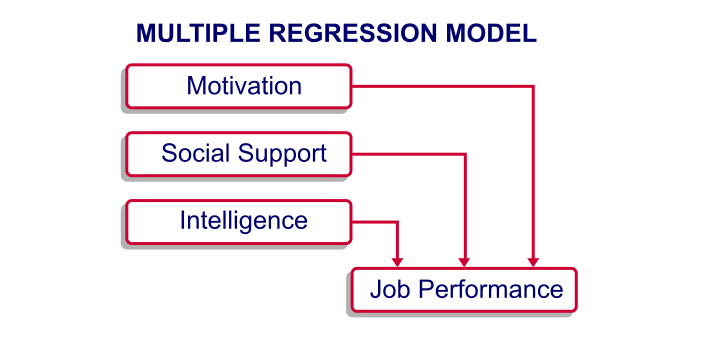
At this point, my model doesn't really get me anywhere; although the model makes intuitive sense, we don't know if it corresponds to reality. Besides, the model suggests that my predictors (IQ, motivation and social support) relate to job performance but it says nothing about how strong these presumed relations are. In essence, regression analysis provides numeric estimates of the strengths of such relations.
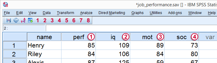
In order to use regression analysis, we need data on the four variables (1 criterion and 3 predictors) in our model. We therefore have our employees take some tests that measure these. Part of the raw data we collect are shown below.

Multiple Regression - Raw Data

Multiple Regression - Meaning Data

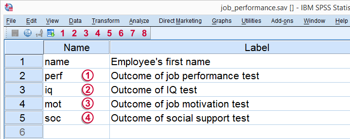
The meaning of each variable in our data is illustrated by the figure below.

Regarding the scores on these tests, tests , and have scores ranging from 0 (as low as possible) through 100 (as high as possible).
IQ has an average of 100 points with a standard deviation of 15 points in an average population; roughly, we describe a score of 70 as very low, 100 as normal and 130 as very high.

Multiple Regression - B Coefficients

Now that we collected the necessary data, we have our software (SPSS or some other package) run a multiple regression analysis on them. The main result is shown below.

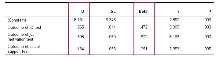
In order to make things a bit more visual, we added the b coefficients to our model overview, which is illustrated below. (We'll get to the beta coefficients later.)

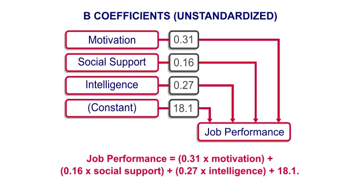
Note that the model now quantifies the strengths of the relations we presume. Precisely, the model says that Job performance = (0.31 x motivation) +
(0.16 x social support) + (0.27 x intelligence) + 18.1. In our model, 18.1 is a baseline score that's unrelated to any other variables. It's a constant over respondents, which means that it's the same 18.1 points for each respondent.
The formula shows how job performance is estimated: we add up each of the predictor scores after multiplying them with some number. These numbers are known as the b coefficients or unstandardized regression coefficients: a B coefficient indicates how many units the criterion changes for a one unit increase on a predictor, everything else equal. In this case, “units” may be taken very literally as the units of measurement of the variables involved. These can be meters, dollars, hours or -in our case- points scored on various tests.
For example, a 1 point increase on our motivation test is associated with a 0.31 points increase on our job performance test. This means that -on average- respondents who score 1 point higher on motivation score 0.31 points higher on job performance. We'll get back to the b coefficients in a minute.

Multiple Regression - Linearity

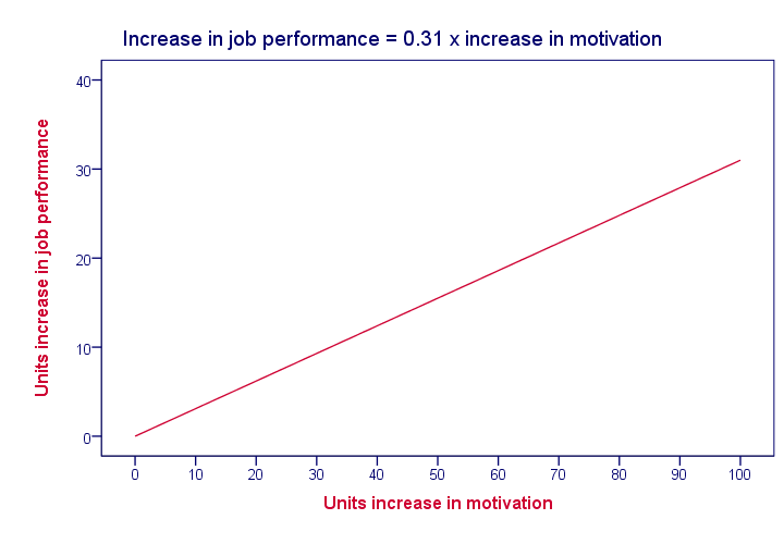
Unless otherwise specified, “multiple regression” normally refers to univariate linear multiple regression analysis. “Univariate” means that we're predicting exactly one variable of interest. “Linear” means that the relation between each predictor and the criterion is linear in our model. For instance, the figure below visualizes the assumed relation between motivation and job performance.

Keep in mind that linearity is an assumption that may or may not hold. For instance, the actual relation between motivation and job performance may just as well be non linear as shown below.

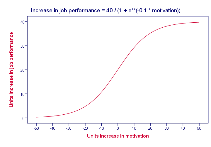
In practice, we often assume linearity at first and then inspect some scatter plots for signs of any non linear relations.

Multiple Regression - Beta Coefficients

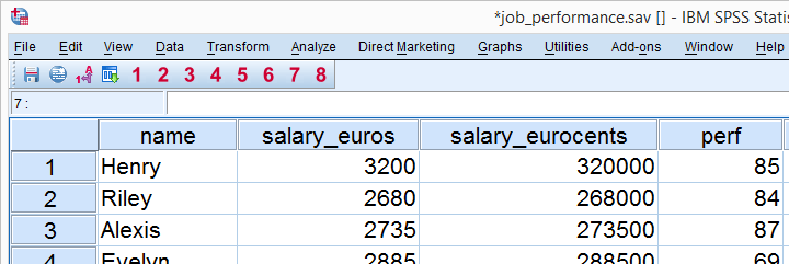
The b coefficients are useful for estimating job performance, given the scores on our predictors. However, we can't always use them for comparing the relative strengths of our predictors because they depend on the scales of our predictors.
That is, if we'd use salary in Euros as a predictor, then replacing it by salary in Euro cents would decrease the B coefficient by a factor 100; if a 1 Euro increase in salary corresponds to a 2.3 points increase in job performance, then a one Euro cent increase corresponds to a (2.3 / 100 =) 0.023 points increase. However, you probably sense that changing Euros to Euro cents doesn't make salary a “stronger” predictor.

The solution to this problem is to standardize the criterion and all predictors; we transform them to z-scores. This gives all variables the same scale: the number of standard deviations below or above the variable’ s mean.
If we rerun our regression analysis using these z-scores, we get b coefficients that allow us to compare the relative strengths of the predictors. These standardized regression coefficients are known as the beta coefficients. Beta coefficients are b coefficients obtained by running regression on standardized variables. The next figure shows the beta coefficients obtained from our multiple regression analysis.

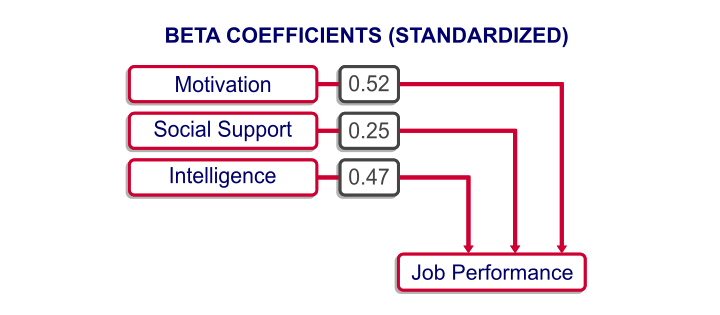
A minor note here is that the aforementioned constant has been left out of the figure. After standardizing all variables, it's always zero because z scores always have a meann of zero by definition.

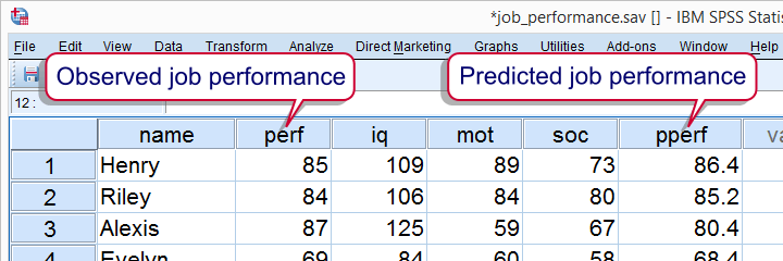
Multiple Regression - Predicted Values

Right, now back to the b coefficients: note that we can use the b coefficients to predict job performance for each respondent. For instance, let's consider the scores of our first respondent, Henry, which are shown below.

For Henry, our regression model states that job performance = (109 x 0.27) + (89 x 0.31) + (73 x 0.16) + 18.1 = 86.8. That is, Henry has a predicted value for job performance of 86.8. This is the job performance score that Henry should have according to our model. However, since our model is just an attempt to approximate reality, the predicted values usually differ somewhat from the actual values in our data. We'll now explore this issue a bit further.

Multiple Regression - R Square

Instead of manually calculating model predicted values for job performance, we can have our software do it for us. After doing so, each respondent will have two job performance scores: the actual score as measured by our test and the value our model comes up with. Part of the result is shown below.

Now, if our model performs well, these two scores should be pretty similar for each respondent. We'll inspect to which extent this is the case by creating a scatterplot as shown below.

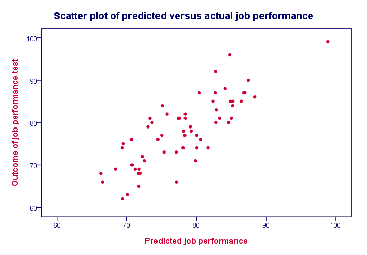
We see a strong linear relation between the actual and predicted values. The strength of such a relation is normally expressed as a correlation. For these data, there is a correlation of 0.81 between the actual and predicted job performance scores. However, we often report the square of this correlation, known as R square, which is 0.65. R square is the squared (Pearson) correlation between
predicted and actual values. We're interested in R square because it indicates how well our model is able to predict a variable of interest. An R square value of 0.65 like we found is generally considered very high; our model does a great job indeed!

Multiple Regression - Adjusted R Square

Remember that the b coefficients allow us to predict job performance, given the scores on our predictors. So how does our software come up the b coefficients we reported? Why did it choose 0.31 for motivation instead of, say, 0.21 or 0.41? The basic answer is that it calculates the b coefficients that lead to predicted values that are as close to the actual values as possible. This means that the software calculates the b coefficients that maximize R square for our data.
Now, assuming that our data are a simple random sample from our target population, they'll differ somewhat from the population data due to sampling error. Therefore, optimal b coefficients for our sample are not optimal for our population. This means that we'd also find a somewhat lower R square value if we'd use our regression model on our population. Adjusted R square is an estimate for the population R square if we'd use our sample regression model on our population. Adjusted R square gives a more realistic indication of the predictive power of our model whereas R square is overoptimistic. This decrease in R square is known as shrinkage and becomes worse with smaller samples and a larger number of predictors.

Multiple Regression - Final Notes

This tutorial aims to give a quick explanation of multiple regression basics. In practice, however, more issues are involved such as homoscedasticity and multicollinearity. These are beyond the scope of this tutorial but will be given separate tutorials in the near future.