A Spearman rank correlation is a number between -1 and +1 that indicates to what extent 2 variables are monotonously related.

• Spearman Correlation - Example
• Spearman Rank Correlation - Basic Properties
• Spearman Rank Correlation - Assumptions
• Spearman Correlation - Formulas and Calculation
• Spearman Rank Correlation - Software

Spearman Correlation - Example

A sample of 1,000 companies were asked about their number of employees and their revenue over 2018. For making these questions easier, they were offered answer categories. After completing the data collection, the contingency table below shows the results.

The question we'd like to answer is is company size related to revenue? A good look at our contingency table shows the obvious: companies having more employees typically make more revenue. But note that this relation is not perfect: there's 60 companies with 1 employee making $50,000 - $99,999 while there's 89 companies with 2-5 employees making $0 - $49,999. This relation becomes clear if we visualize our results in the chart below.

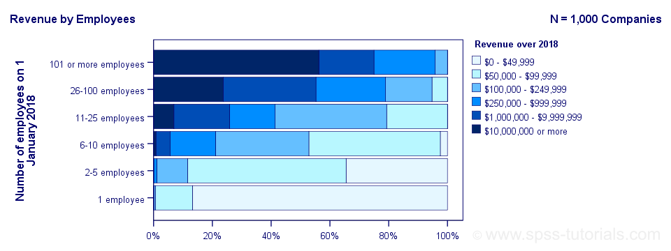
The chart shows an undisputable positive monotonous relation between size and revenue: larger companies tend to make more revenue than smaller companies. Next question. How strong is the relation? The first option that comes to mind is computing the Pearson correlation between company size and revenue. However, that's not going to work because we don't have company size or revenue in our data. We only have size and revenue categories. Company size and revenue are ordinal variables in our data: we know that 2-5 employees is larger than 1 employee but we don't know how much larger.
So which numbers can we use to calculate how strongly ordinal variables are related? Well, we can assign ranks to our categories as shown below.

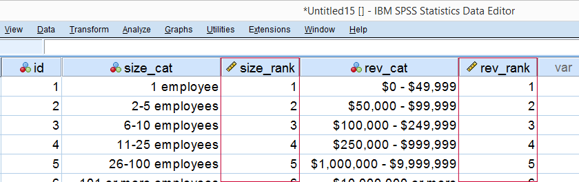
As a last step, we simply compute the Pearson correlation between the size and revenue ranks. This results in a Spearman rank correlation (Rs) = 0.81. This tells us that our variables are strongly monotonously related. But in contrast to a normal Pearson correlation, we do not know if the relation is linear to any extent.

Spearman Rank Correlation - Basic Properties

Like we just saw, a Spearman correlation is simply a Pearson correlation computed on ranks instead of data values or categories. This results in the following basic properties:

• Spearman correlations are always between -1 and +1;
• Spearman correlations are suitable for all but nominal variables. However, when both variables are either metric or dichotomous, Pearson correlations are usually the better choice;
• Spearman correlations indicate monotonous -rather than linear- relations;
• Spearman correlations are hardly affected by outliers. However, outliers should be excluded from analyses instead of determine whether Spearman or Pearson correlations are preferable;
• Spearman correlations serve the exact same purposes as Kendall’s tau.

Spearman Rank Correlation - Assumptions

• The Spearman correlation itself only assumes that both variables are at least ordinal variables. This excludes all but nominal variables.
• The statistical significance test for a Spearman correlation assumes independent observations or -precisely- independent and identically distributed variables.

Spearman Correlation - Example II

A company needs to determine the expiration date for milk. They therefore take a tiny drop each hour and analyze the number of bacteria it contains. The results are shown below.

For bacteria versus time,

• the Pearson correlation is 0.58 but
• the Spearman correlation is 1.00.

There is a perfect monotonous relation between time and bacteria: with each hour passed, the number of bacteria grows. However, the relation is very non linear as shown by the Pearson correlation.
This example nicely illustrates the difference between these correlations. However, I'd argue against reporting a Spearman correlation here. Instead, model this curvilinear relation with a (probably exponential) function. This'll probably predict the number of bacteria with pinpoint precision.

Spearman Correlation - Formulas and Calculation

First off, an example calculation, exact significance levels and critical values are given in this Googlesheet (shown below).

Right. Now, computing Spearman’s rank correlation always starts off with replacing scores by their ranks (use mean ranks for ties). Spearman’s correlation is now computed as the Pearson correlation over the (mean) ranks.

Alternatively, compute Spearman correlations with $$R_s = 1 - \frac{6\cdot \Sigma \;D^2}{n^3 - n}$$
where \(D\) denotes the difference between the 2 ranks for each observation.

For reasonable sample sizes of N ≥ 30, the (approximate) statistical significance uses the t distribution. In this case, the test statistic $$T = \frac{R_s \cdot \sqrt{N - 2}}{\sqrt{1 - R^2_s}}$$
follows a t-distribution with $$Df = N - 2$$
degrees of freedom.

This approximation is inaccurate for smaller sample sizes of N < 30. In this case, look up the (exact) significance level from the table given in this Googlesheet. These exact p-values are based on a permutation test that we may discuss some other time. Or not.

Spearman Rank Correlation - Software

Spearman correlations can be computed in Googlesheets or Excel but statistical software is a much easier option. JASP -which is freely downloadable- comes up with the correct Spearman correlation and its significance level as shown below.

SPSS also comes up with the correct correlation. However, its significance level is based on the t-distribution: $$t = \frac{0.77\cdot\sqrt{4}}{\sqrt{(1 - 0.77^2)}} = 2.42$$
and $$t(4) = 2.42,\;p = 0.072 $$
Again, this approximation is only accurate for larger sample sizes of N ≥ 30. For N = 6, it is wildly off as shown below.

Thanks for reading.