By default, every case in your data counts as a single case. However, you can have each case count as more or less than one case as well. This is called weighting.
For instance, the first case in your data may count as 2 cases and the second one as .5 cases. These numbers, the case weights, are contained in a weight variable. Running WEIGHT BY [...] tells SPSS to treat the values of some weight variable as the active case weights. Note that the status bar informs you whether weighting is in effect or not.

SPSS Weight - Basic Use
Similarly to SPLIT FILE and FILTER, WEIGHT has three main commands.
WEIGHT BY [...].switches a weight variable on. If a weight variable is already in effect, it can be used for setting a different variable as the active case weights.SHOW WEIGHT.shows which variable is currently used as the weight variable.WEIGHT OFF.switches the case weights off. After doing so, every case counts as a single case again.
SPSS Weight - Caveats
- In contrast to
SPLIT FILEandFILTER, the active weight variable is saved with the data. So when you start SPSS and open a data file, a weight variable may already be in effect. - An active weight variable does not only affect the output that's generated. Some data modifications are also influenced by case weights (most notably
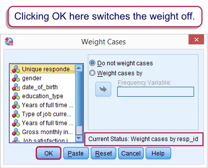
AGGREGATE). - Some users inspect which weight variable is in effect from the menu. When seeing current status: Weight cases (...), they agree with that and click . However, this turns the weight variable off.
 Accidentally turning case weights off
Why Would you Weight Cases?
The main scenarios in which you'll want to weight your cases are the following:
- Your sample is not representative for the population you're investigating. For example, you may know that 50% of your target population consist of females but you have 80% females in your sample. In this case you can weight down these 80% of females to 50% of your sample by assigning case weights of .625 to them. Similarly, you can weight up the 20% male respondents to 50% of your sample as well by using weights of 2.5.
Note that these weights don't correspond to the numbers of observations actually made. In this scenario, weights typically have a mean of 1 so the weighted sample size is exactly equal to the unweighted sample size. We'll demonstrate this scenario with the example below. - In some cases you only have aggregated data. A typical example is a contingency table ("crosstab") presented in a book or article. In this case, case weights will al be positive integers. In this case, weights correspond to the numbers of observations that were actually made.
- You may trick SPSS by using weights in some cases but this is beyond the scope of this tutorial.
SPSS Weight - Example
“We held a small survey on income. Unfortunately, 80% of our respondents are female while this is 50% of our target population. That is, our sample is not representative for our population because female respondents are overrepresented.”
Running the syntax below creates these data and computes mean incomes for male, female and all respondents.
data list free / case_weight gender income.
begin data
2.5, 0, 2200, 2.5, 0, 2000, 0.625, 1, 2700, 0.625, 1, 2300, 0.625, 1, 2400, 0.625, 1, 2700, 0.625, 1, 2400, 0.625, 1, 2300, 0.625, 1, 2500, 0.625, 1, 2200
end data.
value labels gender 0 'Male' 1 'Female'.
*2. Unweighted mean incomes.
means income by gender.
Biased Estimate for Unweighted Cases
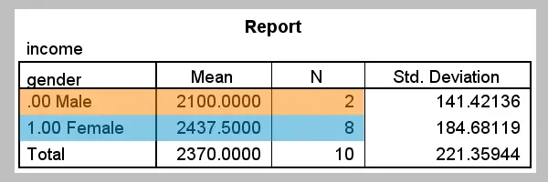
 Female respondents overrepresented and having higher incomes
Note in the screenshot above that female respondents have higher average incomes and are overrepresented as well. The result of this is that the estimated mean income for the entire target population (€ 2370,-) is biased upwards. We can correct this by weighting our respondents as described earlier. The syntax below demonstrates how to do so.
weight by case_weight.
show weight.
means income by gender.
*4. Switch off weight and do quick check on it.
weight off.
show weight.
Unbiased Estimate for Weighted Cases
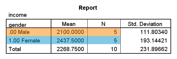
 Females and males equally represented when weight in effect
In the screenshot above, first take a look at the sample sizes. They're now equal for females and males, thus rendering the sample representative of the target population with regard to gender. Also note that the total sample size is still 10. This is because the average case weight is exactly one. Second, the estimated mean income for our target population is now € 2268,75-. This is because we correct for the aforementioned upwards bias by weighting.
 SPSS TUTORIALS
THIS TUTORIAL HAS 13 COMMENTS:
By Greta on March 25th, 2015
Nice and straightforward. I wish it went farther or there were follow-up tutorials on weighting topics such as using weighted data in statistical tests.
By Ruben Geert van den Berg on March 30th, 2015
For a general discussion, you might want to consult the International Handbook of Survey Methodology by Joop Hox and friends. Regarding SPSS, there's the Complex Samples option that deals with probability weights as well as samples from (very) finite populations and cluster/stratified samples.
In any case, these are rather specialized topics and we agree they are underrated and undercovered by most standard texts.
By Njobvu Michael on July 7th, 2015
I have liked this site and very much helping me with the analysis. I am getting the right full details on how to go about with the SPSS. Will give me more insight into syntaxes? I'm going to really appreciate your help. Thanks.
By Ruben Geert van den Berg on July 7th, 2015
Thank you for the compliment. Regarding your question, all our tutorials are syntax based so I'm sure you'll pick it up along your way. For getting started with syntax we have an SPSS Syntax Basics Tutorial, which is followed up by SPSS Syntax Shortening.
By Menzi Bolaji on April 16th, 2016
thanks, its a very helpful site.