A magazine wants to improve their customer satisfaction. They surveyed some readers on  their overall satisfaction as well as
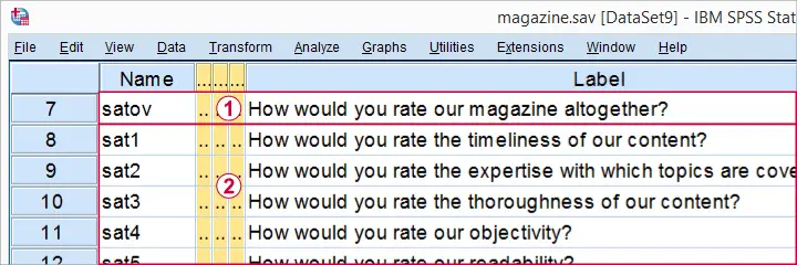
 satisfaction with some quality aspects. Their basic question is
“which aspects have most impact on customer satisfaction?”
We'll try to answer this question with regression analysis. Overall satisfaction is our dependent variable (or criterion) and the quality aspects are our independent variables (or predictors).
satisfaction with some quality aspects. Their basic question is
“which aspects have most impact on customer satisfaction?”
We'll try to answer this question with regression analysis. Overall satisfaction is our dependent variable (or criterion) and the quality aspects are our independent variables (or predictors).
These data -downloadable from magazine_reg.sav- have already been inspected and prepared in Stepwise Regression in SPSS - Data Preparation.
Preliminary Settings
Our data contain a FILTER variable which we'll switch on with the syntax below. We also want to see both variable names and labels in our output so we'll set that as well.
filter by filt1.
*2. Show variable names and labels in output.
set tvars both.
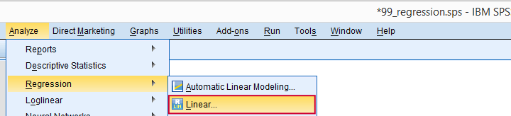
SPSS ENTER Regression
We'll first run a default linear regression on our data as shown by the screenshots below.
Let's now fill in the dialog and subdialogs as shown below.
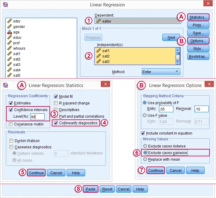
Note that we usually select  because it uses as many cases as possible for computing the correlations on which our regression is based.
Clicking results in the syntax below. We'll run it right away.
SPSS ENTER Regression - Syntax
REGRESSION
/MISSING PAIRWISE
/STATISTICS COEFF CI(99) OUTS R ANOVA COLLIN TOL
/CRITERIA=PIN(.05) POUT(.10)
/NOORIGIN
/DEPENDENT satov
/METHOD=ENTER sat1 sat2 sat3 sat4 sat5 sat6 sat7 sat8 sat9.
SPSS ENTER Regression - Output
In our output, we first inspect our coefficients table as shown below.
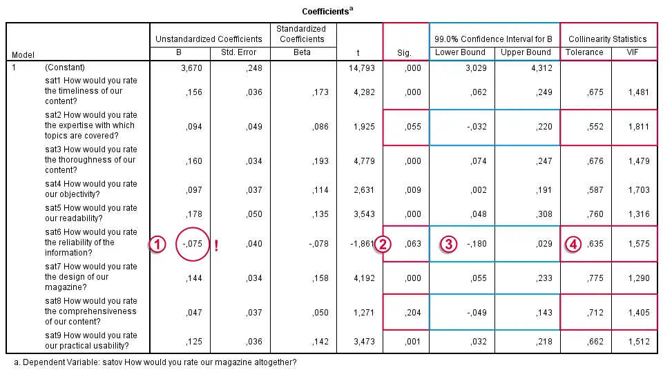
Some things are going dreadfully wrong here:
The b-coefficient of -0.075 suggests that lower “reliability of information” is associated with higher satisfaction. However, these variables have a positive correlation (r = 0.28 with a p-value of 0.000).
This weird b-coefficient is not statistically significant: there's a 0.063 probability of finding this coefficient in our sample if it's zero in the population. This goes for some other predictors as well.
This problem is known as multicollinearity: we entered too many intercorrelated predictors into our regression model. The (limited) r square gets smeared out over 9 predictors here. Therefore, the unique contributions of some predictors become so small that they can no longer be distinguished from zero.
 The confidence intervals confirm this: it includes zero for three b-coefficients.
 A rule of thumb is that Tolerance < 0.10 indicates multicollinearity. In our case, the Tolerance statistic fails dramatically in detecting multicollinearity which is clearly present. Our experience is that this is usually the case.
Resolving Multicollinearity with Stepwise Regression
A method that almost always resolves multicollinearity is stepwise regression. We specify which predictors we'd like to include. SPSS then inspects which of these predictors really contribute to predicting our dependent variable and excludes those who don't.
Like so, we usually end up with fewer predictors than we specify. However, those that remain tend to have solid, significant b-coefficients in the expected direction: higher scores on quality aspects are associated with higher scores on satisfaction. So let's do it.
SPSS Stepwise Regression - Syntax
We copy-paste our previous syntax and set METHOD=STEPWISE in the last line. Like so, we end up with the syntax below. We'll run it and explain the main results.
REGRESSION
/MISSING PAIRWISE
/STATISTICS COEFF OUTS CI(99) R ANOVA
/CRITERIA=PIN(.05) POUT(.10)
/NOORIGIN
/DEPENDENT satov
/METHOD=stepwise sat1 sat2 sat3 sat4 sat5 sat6 sat7 sat8 sat9.
SPSS Stepwise Regression - Variables Entered
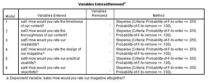
This table illustrates the stepwise method: SPSS starts with zero predictors and then adds the strongest predictor, sat1, to the model if its b-coefficient in statistically significant (p < 0.05, see last column).
It then adds the second strongest predictor (sat3). Because doing so may render previously entered predictors not significant, SPSS may remove some of them -which doesn't happen in this example.
This process continues until none of the excluded predictors contributes significantly to the included predictors. In our example, 6 out of 9 predictors are entered and none of those are removed.
SPSS Stepwise Regression - Model Summary
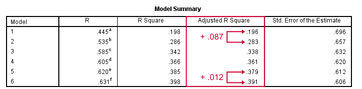
SPSS built a model in 6 steps, each of which adds a predictor to the equation. While more predictors are added, adjusted r-square levels off: adding a second predictor to the first raises it with 0.087, but adding a sixth predictor to the previous 5 only results in a 0.012 point increase. There's no point in adding more than 6 predictors.
Our final adjusted r-square is 0.39, which means that our 6 predictors account for 39% of the variance in overall satisfaction. This is somewhat disappointing but pretty normal in social science research.
SPSS Stepwise Regression - Coefficients
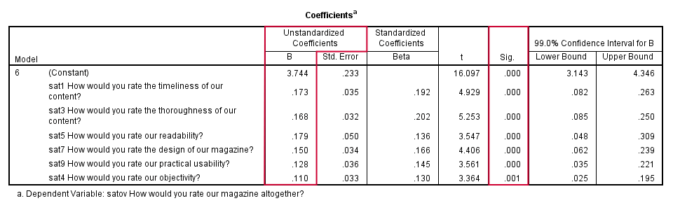
In our coefficients table, we only look at our sixth and final model. Like we predicted, our b-coefficients are all significant and in logical directions. Because all predictors have identical (Likert) scales, we prefer interpreting the b-coefficients rather than the beta coefficients. Our final model states that
satov’ = 3.744 + 0.173 sat1 + 0.168 sat3 + 0.179 sat5
+ 0.150 sat7 + 0.128 sat9 + 0.110 sat4
Our strongest predictor is sat5 (readability): a 1 point increase is associated with a 0.179 point increase in satov (overall satisfaction). Our model doesn't prove that this relation is causal but it seems reasonable that improving readability will cause slightly higher overall satisfaction with our magazine.
THIS TUTORIAL HAS 15 COMMENTS:
By Muhammad ilyas on January 12th, 2017
good one
By Jon Peck on March 3rd, 2017
My main point is that users need to be aware of the problems with stepwise so as not to be mislead by the results. It is simple and is useful as an exploratory technique.
It might be useful to point out that REGRESSION supports a mixture of entry methods, so some variables can be forced into the equation while others are subject to stepwise selection.
Another technique I like is the STATS RELIMP extension command (under Regression). It shows you not only which variables matter the most but how their coefficients vary across models with different numbers of variables.
As for pairwise deletion, while it maximizes data use, it also leads to biased coefficient standard errors.
By Muhammad Asad Khan on March 11th, 2017
This article is very informative
By Ruben Geert van den Berg on March 12th, 2017
Thank you. We published a more detailed -and I think better- example of a similar analysis last week: SPSS Stepwise Regression – Example 2. You might like that one too.
By meche on May 22nd, 2017
this is good