Contents

• Cronbach’s Alpha - Quick Definition
• SPSS Cronbach’s Alpha Output
• Increase Cronbach’s Alpha by Removing Items
• Cronbach’s Alpha is Negative
• There are too Few Cases (N = 0) for the Analysis
• APA Reporting Cronbach’s Alpha

Introduction

A psychology faculty wants to examine the reliability of a personality test. They therefore have a sample of N = 90 students fill it out. The data thus gathered are in big-5.sav, partly shown below.

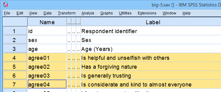
As suggested by the variable names, our test attempts to measure the “big 5” personality traits. For other data files, a factor analysis is often used to find out which variables measure which subscales.

Anyway. Our main research question is: what are the reliabilities for these 5 subscales as indicated by Cronbach’s alpha? But first off: what's Cronbach’s alpha anyway?

Cronbach’s Alpha - Quick Definition

Cronbach’s alpha is the extent to which the sum over 2(+)
variables measures a single underlying trait. More precisely, Cronbach’s alpha is the proportion of variance of such a sum score that can be accounted for by a single trait. That is, it is the extent to which a sum score reliably measures something and (thus) the extent to which a set of items consistently measure “the same thing”.

Cronbach’s alpha is therefore known as a measure of reliability or internal consistency. The most common rules of thumb for it are that

• Cronbach’s alpha ≥ 0.80 is good and
• Cronbach’s alpha ≈ 0.70 may or may not be just acceptable.

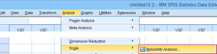
SPSS Reliability Dialogs

In SPSS, we get Cronbach’s alpha from Analyze Scale Reliability Analysis... as shown below.

For analyzing the first subscale, agreeableness, we fill out the dialogs as shown below.

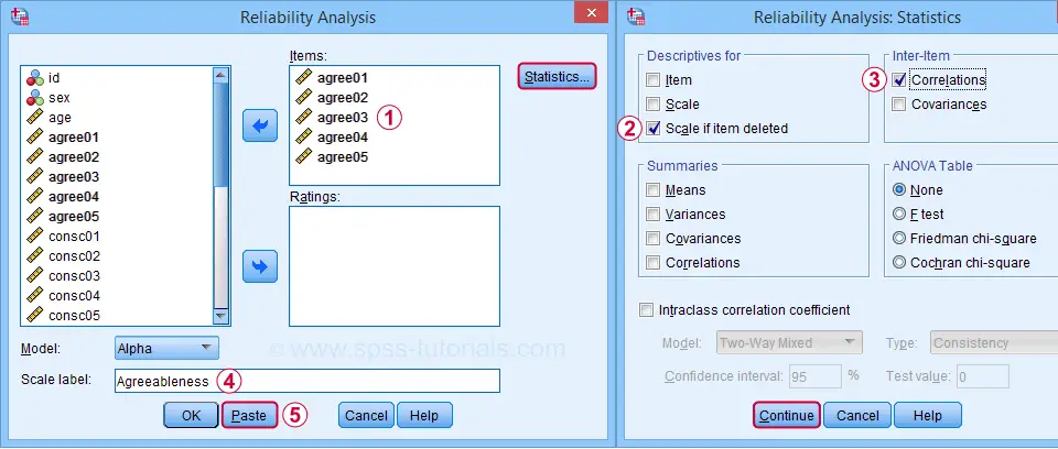
Clicking Paste results in the syntax below. Let's run it.

SPSS Cronbach’s Alpha Output I

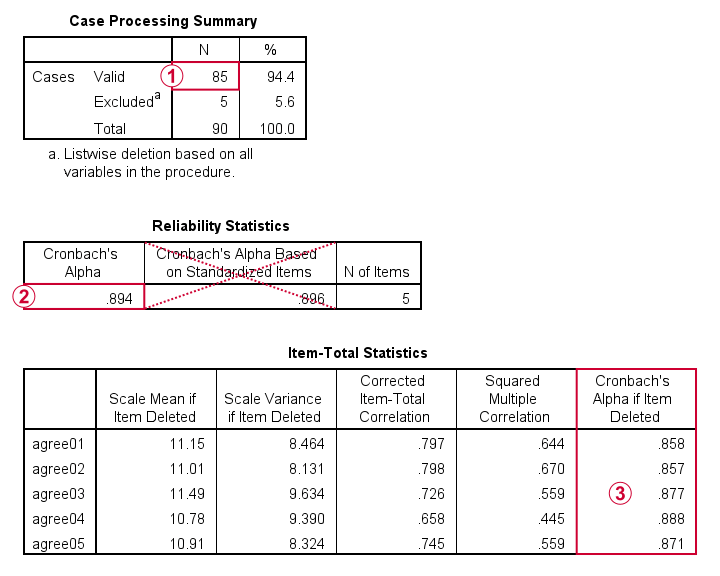
For reliability, SPSS only offers listwise exclusion of missing values: all results are based only on N = 85 cases having zero missing values on our 5 analysis variables or “items”.

Cronbach’s alpha = 0.894. You can usually ignore Cronbach’s Alpha Based on Standardized Items: standardizing variables into z-scores prior to computing scale scores is rarely -if ever- done.

Finally, excluding a variable from a (sub)scale may increase Cronbach’s Alpha. That's not the case in this table: for each item, Cronbach’s Alpha if Item Deleted is lower than the α = 0.894 based on all 5 items.

We'll now run the exact same analysis for our second subscale, conscientiousness. Doing so results in the syntax below.

Increase Cronbach’s Alpha by Removing Items

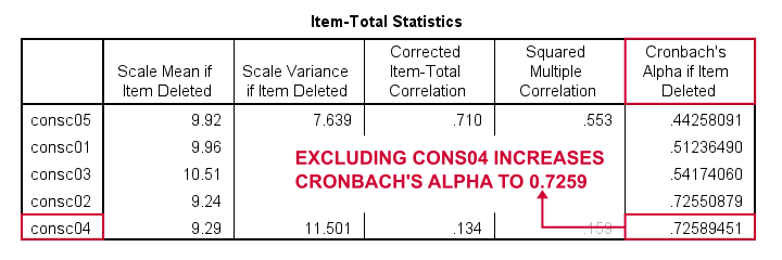
For the conscientiousness subscale, Cronbach’s alpha = 0.658, which is pretty poor. However, note that Cronbach’s Alpha if Item Deleted = 0.726 for both consc02 and consc04.

Since removing either item should result in α ≈ 0.726, we're not sure which should be removed first. Two ways to find out are

• increasing the decimal places or (better)
• sorting the table by its last column.

As you probably saw, we already did both with the following OUTPUT MODIFY commands:

It turns out that removing consc04 increases alpha slightly more than consc02. The preferred way for doing so is to simply copy-paste the previous RELIABILITY command, remove consc04 from it and rerun it.

After doing so, Cronbach’s alpha = 0.724. It's not exactly the predicted 0.726 because removing consc04 increases the sample size to N = 84. Note that we can increase α even further to 0.814 by removing consc02 as well. The syntax below does just that.

Note that Cronbach’s alpha = 0.814 if we compute our conscientiousness subscale as the sum or mean over consc01, consc03 and consc05. Since that's fine, we're done with this subscale.

Let's proceed with the next subscale: extraversion. We do so by running the exact same analysis on extra01 to extra05, which results in the syntax below.

Cronbach’s Alpha is Negative

As shown below, Cronbach’s alpha = -0.663 for the extraversion subscale. This implies that some correlations among items are negative (second table, below).

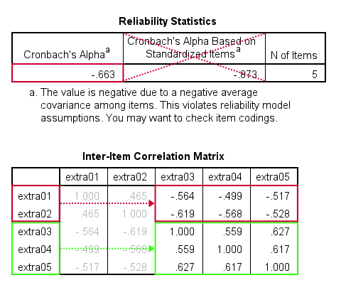
All extraversion items are coded similarly: they have identical value labels so that's not the problem. The problem is that some items measure the opposite of the other items as shown below.

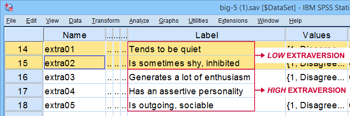
The solution is to simply reverse code such “negative items”: we RECODE these 2 items and adjust their value/variable labels with the syntax below.

Rerunning the exact same reliability analysis as previous now results in Cronbach’s alpha = 0.857 for the extraversion subscale.

So let's proceed with the neuroticism subscale. The syntax below runs our default reliability analysis on neur01 to neur05.

There are too Few Cases (N = 0) for the Analysis

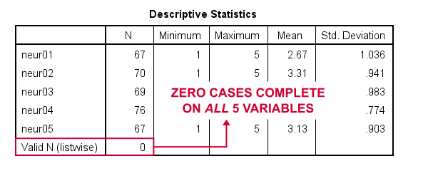
Note that our last command doesn't result in any useful tables. We simply get the warning that

as shown below.

The 3 most likely causes for this problem are that

• one or more variables contains only missing values;
• an incorrect FILTER filters out all cases in the data;
• missing values are scattered over numerous analysis variables.

A very quick way to find out is running a minimal DESCRIPTIVES command as in descriptives neur01 to neur05. Upon doing so, we learn that each variable has N ≥ 67 but valid N (listwise) = 0.

So what we really want here, is to use pairwise exclusion of missing values. For some dumb reason, that's not included in SPSS. However, doing it manually isn't as hard as it seems.

Cronbach’s Alpha with Pairwise Exclusion of Missing Values

We'll start off with the formula for Cronbach’s alpha, which is

$$Cronbach’s\;\alpha = \frac{k^2 \overline{S_{xy}}}{\Sigma S^2_x + 2 \Sigma S_{xy}}$$

where

• \(k\) denotes the number of items;
• \(S_{xy}\) denotes the covariance between each pair of different items;
• \(S^2_x\) denotes the sample variance for each item.

Note that a pairwise covariance matrix contains all statistics used by this formula. It is easily obtained via the regression syntax below:

Next, we copy the result into this Googlesheet. Finally, a handful of very simple formulas tell us that α = 0.889.

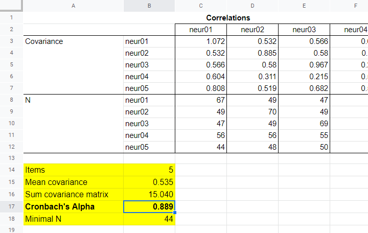
Now, which sample size should we report for this subscale? I propose you follow the conventions for pairwise regression here and report the smallest pairwise N which results in N = 44 for this analysis. Again, note that the formula for finding this minimum over a block of cells is utterly simple.

APA Reporting Cronbach’s Alpha

The table below shows how to report Cronbach’s alpha in APA style for all subscales.

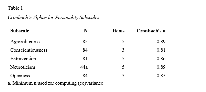
This table contains the actual results from big-5.sav so you can verify that your analyses correspond to mine. The easiest way to create this table is to manually copy-paste your final results into Excel. This makes it easy to adjust things such as decimal places and styling.

Thanks for reading.