• Descriptive Statistics - Tables
• Descriptive Statistics - Charts
• Inferential Statistics
• Statistical Significance
• Confidence Intervals

“Statistics” can mean 2 things:

1. the plural of “statistic”, a number or expression that says something about your data or
2. the science of getting useful information from data.

This quick introduction mainly aims at the second meaning. So let's first clarify what we mean by “data” and “useful information”.

Main Components of Data

Although there's exceptions -such as unstructured text or diagonal correlation matrices- the vast majority of data is organized in rectangular grids. This goes for

• SQL tables,
• Excel files,
• .csv or other text files and
• SPSS data files.

All such data grids consist of 4 main components. The figure below illustrates this for a typical SPSS data file.

The data matrix refers to the entire data grid. It holds the actual data but there may be additional tables containing metadata -explanatory information about the actual data.
Variables are usually columns of cells that represent characteristics of our observations (often people).
Observations are usually rows of cells that represent the entities we collected data on.
Values or data points are the contents of the cells that make up both observations and variables.

This hopefully gives you an idea of what we typically mean by “data”. Let's now zoom in on what we mean by “useful information”.

Descriptive Versus Inferential Statistics

Raw data don't usually give a lot of insights that are easily communicated. We get such insights by summarizing and visualizing raw data with statistics. These come in 2 basic types:

1. descriptive statistics simply summarize our data -often in tables and charts;
2. inferential statistics attempt to generalize sample outcomes to (much larger) populations.

Descriptive Statistics - Tables

The first way to get “useful information” from raw data is creating tables with descriptive statistics. The figure below gives an example.

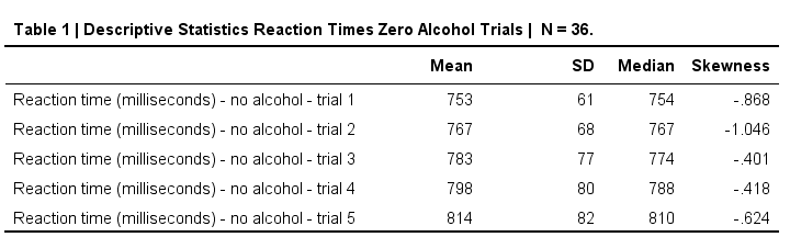
This simple table gives us quite a few insights on our data. For example,

• the mean and median reaction times tend to increase over trials;
• the standard deviations of the reaction times also seem to increase;
• the skewnesses don't show any clear pattern over trials.

Descriptive Statistics - Charts

Charts may convey a high level of insight that can't be matched by just numbers -even though the latter are more exact. The figure below nicely illustrates this point.

Some basic conclusions from this chart are that

• only middle and upper managers have huge salaries and these are hardly related to working hours;
• middle and upper managers work at least some 30 hours per week;
• none of the employees in sales and marketing have high salaries and some work only few hours per week.

Inferential Statistics

Inferential statistics either refers to

• the science of drawing inferences (conclusions) on populations based on samples or
• the plural of inferential statistic, a number or expression that relates a sample outcome to a population.

Two inferential statistics that are particularly important are

• statistical significance and
• confidence intervals.

Both are solutions for the same problem: if our data contain a sample from a much larger population, our sample outcomes tend to differ somewhat from their population counterparts. The figure below illustrates the basic idea.

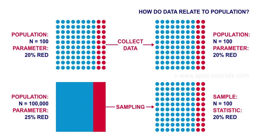
In the first scenario, we're interested in a tiny population of only N = 100. In this case, we can often study the entire population. Neither significance tests nor confidence intervals make any sense here: our data come up with the exact population outcome -a parameter- we're after.
The second scenario involves a population of 100,000 -often way too large to study entirely. So we sample N = 100 respondents. In this case, our sample outcome is likely to be “off” somewhat. That's still better than no information at all but we probably do want to know how much our statistic is likely to be off.
Note that both scenarios result in the exact same data. So just the data aren't enough for drawing the right conclusions: we also need to know our data relate to our population.

Sadly, applied research rarely even mentions which population it's after. On top of that, most textbooks quietly assume that all data hold simple random samples from populations. These are serious flaws with detrimental results: some analysts blindly run statistical tests on population data -utter nonsense as we know by now.
On top of that, most sampling procedures don't even come close to simple random sampling. This may be the single greatest threat to the social sciences. Interestingly, this issue is almost routinely overlooked.

Statistical Significance

Roughly speaking, statistical significance is the probability of finding your data given some null hypothesis. More precisely, statistical significance is the probability of finding at least the (absolute) observed deviation from some null hypothesis. The confusing part is that findings are more “significant” insofar as their statistical significance is lower. We therefore prefer “p-values” instead of “significance”. A general convention is that we reject the null hypothesis if p < 0.05 but this is truly arbitrary. The figure below illustrates a simple significance test.

A sample of N = 100 came up with a proportion of 0.20 -or 20%- for some characteristic. These numbers are descriptive statistics because they simply summarize the sample data.
The null hypothesis is that 25% -a proportion of 0.25- of the entire population has this given characteristic.
If this hypothesis is true, then there's a 0.21 probability of finding at least the absolute observed difference of 0.05. That is, there's a 21% chance that a sample of N = 100 comes up with a proportion between 0.20 and 0.30; these are likely outcomes given our null hypothesis.

Confidence Intervals

A different approach -though not always applicable- are confidence intervals. As a rough definition, confidence interval are ranges of values that enclose some parameter with a given probability. In this case, we estimate some parameter -such as a population mean or proportion- and we also estimate how much we're likely to be off. The figure below gives an example.

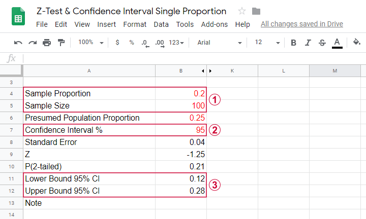
Some sample of N = 100 came up with a proportion of 0.20 for some characteristic. Given this sample outcome, our best guess for the population proportion is also 0.20. But how much is it likely to be off?
We choose to construct an interval that has a 95% probability of enclosing the population proportion.
The interval 0.12 through 0.28 has a 95% likelihood of enclosing the population proportion we're after.

Final Notes

This tutorial very briefly outlined some main lines of thought behind statistics. Obviously, there's way more to explore:

• the z-test we presented nicely illustrates some basics but isn't used very often. For a simple overview of more popular statistical tests, read up on Which Statistical Test Should I Use?
• there's many other -more important- statistics besides the proportions we discussed. Some examples are the mode, median, skewness and standard deviation.
• read up on statistical significance and confidence intervals for understanding these essential concepts more thoroughly.

Right, that'll do for today. Anything missing or unclear? Don't be shy. Please drop us a line.

Thanks for reading!