The Kruskal-Wallis test is an alternative for a one-way ANOVA if the assumptions of the latter are violated. We'll show in a minute why that's the case with creatine.sav, the data we'll use in this tutorial. But let's first take a quick look at what's in the data anyway.
Quick Data Description
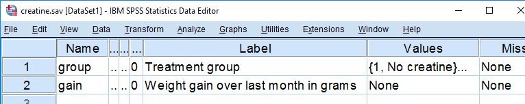
Our data contain the result of a small experiment regarding creatine, a supplement that's popular among body builders. These were divided into 3 groups: some didn't take any creatine, others took it in the morning and still others took it in the evening. After doing so for a month, their weight gains were measured. The basic research question is
does the average weight gain depend on
the creatine condition to which people were assigned?
That is, we'll test if three means -each calculated on a different group of people- are equal. The most likely test for this scenario is a one-way ANOVA but using it requires some assumptions. Some basic checks will tell us that these assumptions aren't satisfied by our data at hand.
Data Check 1 - Histogram
A very efficient data check is to run histograms on all metric variables. The fastest way for doing so is by running the syntax below.
frequencies gain
/formats notable
/histogram.
Histogram Result
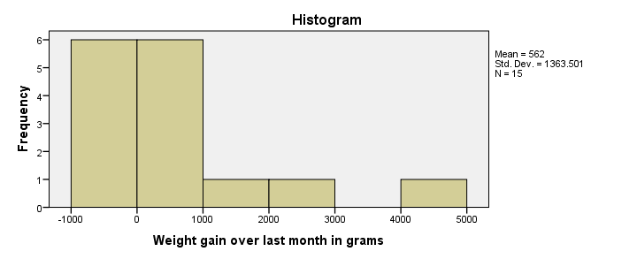
First, our histogram looks plausible with all weight gains between -1 and +5 kilos, which are reasonable outcomes over one month. However, our outcome variable is not normally distributed as required for ANOVA. This isn't an issue for larger sample sizes of, say, at least 30 people in each group. The reason for this is the central limit theorem. It basically states that for reasonable sample sizes the sampling distribution for means and sums are always normally distributed regardless of a variable’s original distribution. However, for our tiny sample at hand, this does pose a real problem.
Data Check 2 - Descriptives per Group
Right, now after making sure the results for weight gain look credible, let's see if our 3 groups actually have different means. The fastest way to do so is a simple MEANS command as shown below.
means gain by group.
SPSS MEANS Output
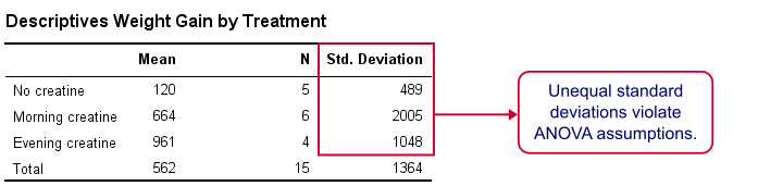
First, note that our evening creatine group (4 participants) gained an average of 961 grams as opposed to 120 grams for “no creatine”. This suggests that creatine does make a real difference.
But don't overlook the standard deviations for our groups: they are very different but ANOVA requires them to be equal.The assumption of equal population standard deviations for all groups is known as homoscedasticity. This is a second violation of the ANOVA assumptions.
Kruskal-Wallis Test
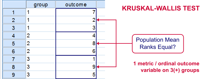
So what should we do now? We'd like to use an ANOVA but our data seriously violates its assumptions. Well, a test that was designed for precisely this situation is the Kruskal-Wallis test which doesn't require these assumptions. It basically replaces the weight gain scores with their rank numbers and tests whether these are equal over groups. We'll run it by following the screenshots below.
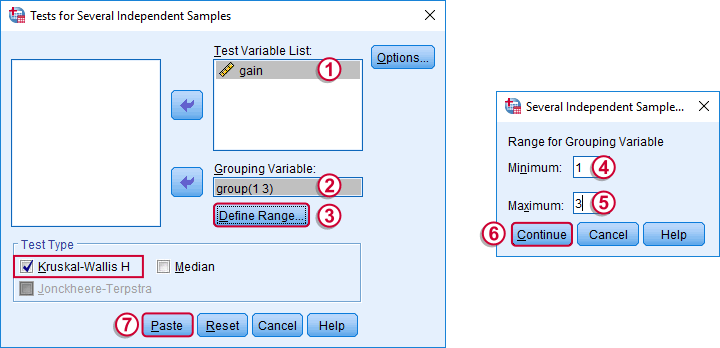
Running a Kruskal-Wallis Test in SPSS
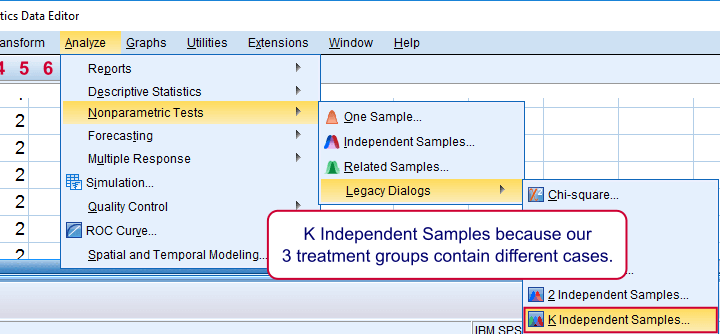
We use if we compare 3 or more groups of cases. They are “independent” because our groups don't overlap (each case belongs to only one creatine condition).
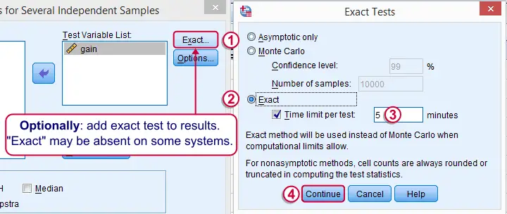
Depending on your license, your SPSS version may or may have the option shown below. It's fine to skip this step otherwise.
SPSS Kruskal-Wallis Test Syntax
Following the previous screenshots results in the syntax below. We'll run it and explain the output.
NPAR TESTS
/K-W=gain BY group(1 3)
/MISSING ANALYSIS.
SPSS Kruskal-Wallis Test Output
We'll skip the “RANKS” table and head over to the “Test Statistics” shown below.
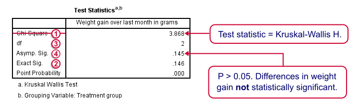
 Our test statistic -incorrectly labeled as “Chi-Square” by SPSS- is known as Kruskal-Wallis H. A larger value indicates larger differences between the groups we're comparing. For our data it's roughly 3.87. We need to know its sampling distribution for evaluating whether this is unusually large.
 Exact Sig. uses the exact (but very complex) sampling distribution of H. However, it turns out that if each group contains 4 or more cases, this exact sampling distribution is almost identical to the (much simpler) chi-square distribution.
 We therefore usually approximate the p-value with a chi-square distribution. If we compare k groups, we have k - 1 degrees of freedom, denoted by df in our output.
 Asymp. Sig. is the p-value based on our chi-square approximation. The value of 0.145 basically means there's a 14.5% chance of finding our sample results if creatine doesn't have any effect in the population at large. So if creatine does nothing whatsoever, we have a fair (14.5%) chance of finding such minor weight gain differences just because of random sampling. If p > 0.05, we usually conclude that our differences are not statistically significant.
Note that our exact p-value is 0.146 whereas the approximate p-value is 0.145. This supports the claim that H is almost perfectly chi-square distributed.
Kruskal-Wallis Test - Reporting
The official way for reporting our test results includes our chi-square value, df and p as in
“this study did not demonstrate any effect from creatine,
H(2) = 3.87, p = 0.15.”
So that's it for now. I hope you found this tutorial helpful. Please let me know by leaving a comment below. Thanks!
THIS TUTORIAL HAS 72 COMMENTS:
By Ruben Geert van den Berg on October 2nd, 2019
Actually, I think it's best to report something like
H(2) = 3.87, p ≈ 0.15.
for the asymptotic significance level where H(2) is shown in SPSS as "chi-quare" and 2 df. Replace ≈ by = for exact significance or mention this in the method section. In any case, these should be very close anyway.
I think I'll adjust the tutorial accordingly.
By Kennedy Mogire on November 25th, 2019
Thanks. I'll need to go over it again. But at least I now have an idea on this test.
By ΕΥΑΓΓΕΛΙΑ ΔΡΑΓΟΥ on December 8th, 2019
Αυτήν η παράμετρος μπορεί να χρησιμοποιηθεί και στην περίπτωση της μη κανονικής κατανομής που δεν μας επιτρέπεται να χρησιμοποιήσουμε την independent t test;;
By Ruben Geert van den Berg on December 9th, 2019
Sorry but this comment is all Greek to me...
By Charu Bansal on April 9th, 2020
Thank you! The explaination was really easy to grasp. Just want to know what to do when our data have two independent variables?