• Normal Distribution - General Formula
• Standard Normal Distribution
• Normal Distribution - Basic Properties
• Finding Probabilities from a Normal Distribution
• Finding Critical Values from an Inverse Normal Distribution
• Are my Variables Normally Distributed?

Definition

The normal distribution is the probability density function defined by
$$f(x) = \frac{1}{\sigma\sqrt{2\pi}}\cdot e^{\dfrac{(x - \mu)^2}{-2\sigma^2}}$$

This results in a symmetrical curve like the one shown below.

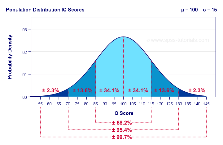
The surface areas under this curve give us the percentages -or probabilities- for any interval of values. Assuming that these IQ scores are normally distributed with a population mean of 100 and a standard deviation of 15 points:

• 34.1% of all people score between 85 and 100 points;
• 15.9% of all people score 115 points or more;
• a random person has a 50% (or 0.50) probability of scoring 100 points or lower.

In statistics, the normal distribution plays 2 important roles:

• a frequency distribution (values over observations): for example, IQ scores are roughly normally distributed over a population of people.
• a sampling distribution (statistic over samples): proportions and means are roughly normally distributed over samples. From this normal distribution we can look up the probability for any observed sample mean or proportion.Strictly, we always look up probabilities for ranges rather than separate outcomes. This is basically statistical significance.

Normal Distribution - General Formula

The general formula for the normal distribution is $$f(x) = \frac{1}{\sigma\sqrt{2\pi}}\cdot e^{\dfrac{(x - \mu)^2}{-2\sigma^2}}$$

where

\(\sigma\) (“sigma”) is a population standard deviation;
\(\mu\) (“mu”) is a population mean;
\(x\) is a value or test statistic;
\(e\) is a mathematical constant of roughly 2.72;
\(\pi\) (“pi”) is a mathematical constant of roughly 3.14.

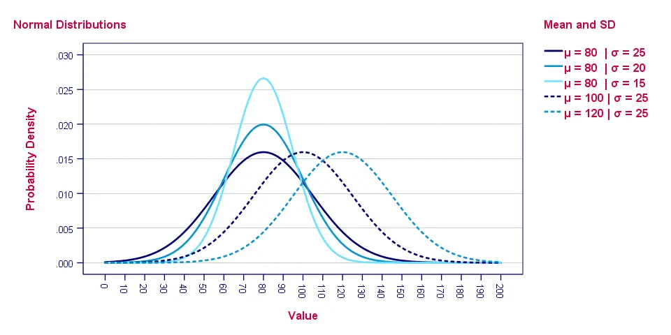
The “normal curve” results from plotting \(f(x)\) -probability density- for a number of \(x\) values. Its horizontal position is set by \(\mu\), its width and height by \(\sigma\). The figure below gives some examples.

As with all probability density functions, the formula does not return probabilities. In order to find these, we need to find the surface areas for ranges of \(x\) values as shown below.

So how to find the probability for any range of values? Well, you could manually compute it from an integral over the normal distribution formula. An easier option, however, is to look it up in Googlesheets as we'll show later on.

Standard Normal Distribution

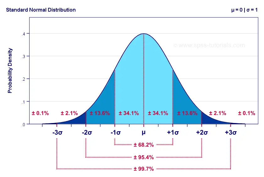
The standard normal distribution is a normal distribution
with μ = 0 and σ = 1. Filling in these numbers into the general formula simplifies it to
$$f(x) = \frac{1}{\sqrt{2\pi}}\cdot e^{\dfrac{x^2}{-2}}$$

The standard normal distribution is the only normal distribution we really need. Why? Well, we can use a normal distribution to look up a probability for \(x\) if

• \(x\) is normally distributed and
• we know its population mean μ and
• we know its population standard deviation σ.

With these 3 numbers we could also compute a z-score: $$z = \frac{x - \mu}{\sigma}$$

The result of doing so is that \(z\) is given a standard of μ = 0 and σ = 1. So if \(x\) follows a normal distribution then \(z\) follows a standard normal distribution.
Converting \(x\) into \(z\) may seem theoretical. However, this is exactly what happens if we run a t-test or a z-test. Keep in mind that computing \(z\) or standardizing values does not “normalize” them in any way. That is, \(z\) only follows a standard normal distribution if \(x\) is normally distributed.

Normal Distribution - Basic Properties

Before we look up some probabilities in Googlesheets, there's a couple of things we should know:

1. the normal distribution always runs from \(-\infty\) to \(\infty\);
2. the total surface area (= probability) of a normal distribution is always exactly 1;
3. the normal distribution is exactly symmetrical around its mean \(\mu\) and therefore has zero skewness;
4. due to its symmetry, the median is always equal to the mean for a normal distribution;
5. the normal distribution always has a kurtosis of zero.

Finding Probabilities from a Normal Distribution

This Googlesheet (read-only) shows how to find probabilities from a normal distribution.

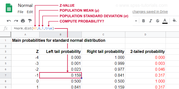
Simply type =norm.dist(a,b,c,true) into some cell and

• replace a by some x or z-value;
• replace b by the population mean μ;
• replace c by the population standard deviation σ.

This results in a left tail probability. Like so, the highlighted example tells us that there's a 0.159 -roughly 16%- probability that z < -1 if z is normally distributed with μ = 0 and σ = 1.

Because the surface area -or total probability- is always 1, we can find any right tail probability with

\(p(X \gt x) = 1 - p(X \lt x)\)
Like so, the probability that z > -1 is (1 - 0.159 =) 0.841.

And what about the probability that x is between -2 and -1? Or -formally- p(-2 < X < -1)? Well,

\(p(x_a \lt X \lt x_b) = p(X \lt x_b) - p(X \lt x_a)\)
so that'll be (0.159 - 0.023 =) 0.136 or 13.6% as shown below.

If you're not sure you master this, try and compute each of the percentages shown above for yourself in an empty Googlesheet.

Finding Critical Values from an Inverse Normal Distribution

• The normal distribution tells us probabilities for ranges of values. These are needed for testing null hypotheses.
• The inverse normal distribution tells us ranges of values for probabilities. These are needed for computing confidence intervals.

This Googlesheet (read-only) illustrates how to find critical values for a normally distributed variable.

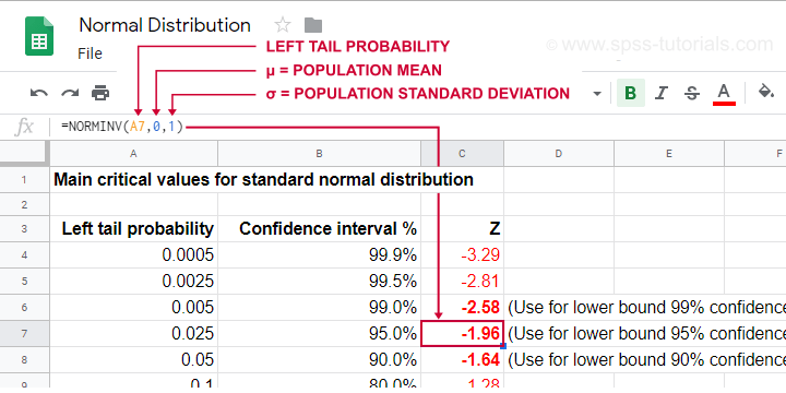
Simply type =norminv(a,b,c) into some cell and

• replace a by the left tail probability;
• replace b by the population mean μ (usually 0);
• replace c by the population standard deviation σ (usually 1);

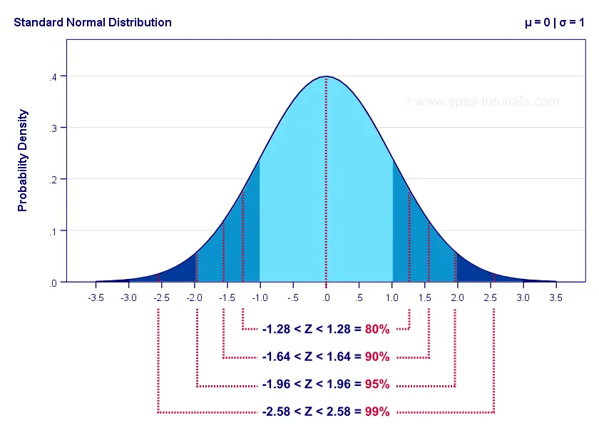
Keep in mind that the probability of not including some parameter is evenly divided over both tails. It is 0.05 for a 95% confidence interval. This 0.05 is divided into a left tail of 0.025 and a right tail of 0.025.
For a standard normal distribution, this results in -1.96 < Z < 1.96. The figure below illustrates how this works.

The exact critical values shown here are all computed in this Googlesheet (read-only).

Are my Variables Normally Distributed?

Many statistical procedures such as ANOVA, t-tests, regression and others require the normality assumption: variables must be normally distributed in the population. This assumption is only needed for small sample sizes of, say, N < 25 or so. For larger samples, the central limit theorem renders most tests robust to violations of normality -but let's discuss that some other day.
Anyway. If a variable is normally distributed in some population, then it should be roughly normally distributed in some sample as well. A first check -simple and solid- is inspecting its frequency distribution from a histogram.

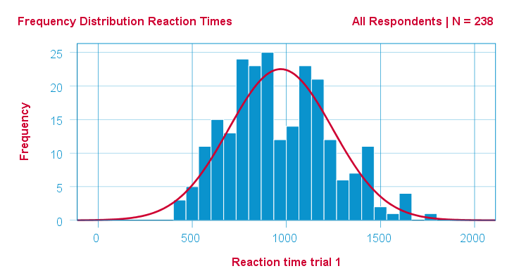
In SPSS, we can very easily add normal curves to histograms. This normal curve is given the same mean and SD as the observed scores. It quickly shows how (much) the observed distribution deviates from a normal distribution.

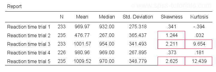
A second check is inspecting descriptive statistics, notably skewness and kurtosis. Some basic properties of the normal distribution are that

• its skewness is exactly 0 and
• its kurtosis is exactly 0 too.

If this is true in some population, then observed variables should probably not have large (absolute) skewnesses or kurtoses. The example table below highlights some striking deviations from this. They suggest that reaction times 2, 3 and 5 are probably not normally distributed in some population.

Last, there's 2 normality tests: statistical tests for evaluating population normality. These are the

• Kolmogorov-Smirnov normality test and the
• Shapiro-Wilk normality test.

Both tests serve the exact same purpose: they test the null hypothesis that a variable is normally distributed in some population.

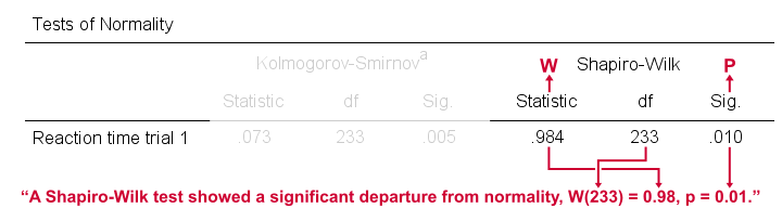
Sadly, both tests have low power in small sample sizes -precisely when normality is really needed. This means they may not reject normality even if it doesn't hold. Like so, they may create a false sense of security and we therefore don't recommend them.

Thanks for reading!