• Z-Test - Simple Example
• Assumptions
• Z-Test Formulas
• Confidence Interval for the Difference between Proportions
• Effect Size I - Cohen’s H
• Z-Tests in Googlesheets

Definition & Introduction

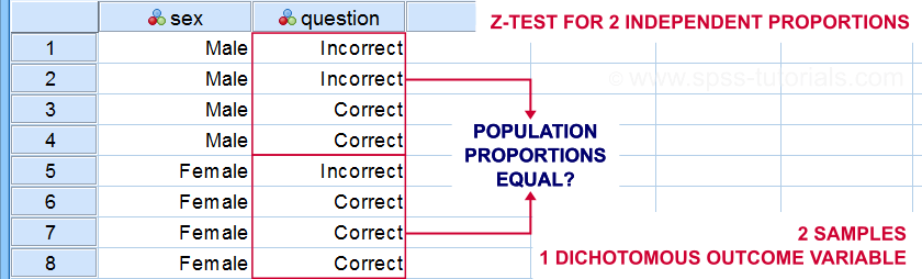
A z-test for 2 independent proportions examines
if some event occurs equally often in 2 subpopulations. Example: do equal percentages of male and female students answer some exam question correctly? The figure below sketches what the data required may look like.

Z-Test - Simple Example

A simple random sample of n = 175 male and n = 164 female students completed 5 exam questions. The raw data -partly shown below- are in this Googlesheet (read-only).

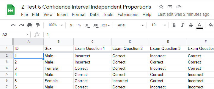
Let's look into exam question 1 first. The raw data on this question can be summarized by the contingency table shown below.

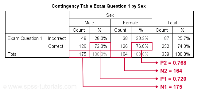
Right, so our contingency table shows the percentages of male and female respondents who answered question 1 correctly. In statistics, however, we usually prefer proportions over percentages. Summarizing our findings, we see that

• a proportion of p1 = 0.720 out of n1 = 175 male students and
• a proportion of p2 = 0.768 out of n2 = 164 female students answered correctly.

In our sample, female students did slightly better than male students. However, sample outcomes typically differ somewhat
from their population counterparts. Even if the entire male and female populations perform similarly, we may still find a small sample difference. This could easily result from drawing random samples of students. The z-test attempts to nullify this hypothesis and thus demonstrate that the populations really do perform differently.

Null Hypothesis

The null hypothesis for a z-test for independent proportions is that the difference between 2 population proportions is zero. If this is true, then the difference between the 2 sample proportions should be close to zero. Outcomes that are very different from zero are unlikely and thus argue against the null hypothesis. So exactly how unlikely is a given outcome? Computing this is fairly easy but it does require some assumptions.

Assumptions

The assumptions for a z-test for independent proportions are

• independent observations and
• sufficient sample sizes.

So what are sufficient sample sizes? Agresti and Franklin (2014)⁴ suggest that the test results are sufficiently accurate if

• \(p_a \cdot n_a \gt 10\),
• \((1-p_a) \cdot n_a \gt 10\),
• \(p_b \cdot n_b \gt 10\),
• \((1-p_b) \cdot n_b \gt 10\)

where

• \(n_a\) and \(n_b\) denote the sample sizes of groups a and b and
• \(p_a\) and \(p_b\) denote the proportions of “successes” in both groups.

Z-Test Formulas

For computing our z-test, we first simply compute the difference between our sample proportions as

$$dif = p1 - p2$$

For our example data, this results in

$$dif = 0.720 - 0.768 = -.048.$$

Now, the null hypothesis claims that both subpopulations have the same proportion of successes. We estimate this as

$$\hat{p} = \frac{p_a\cdot n_a + p_b\cdot n_b}{n_a + n_b}$$

where \(\hat{p}\) is the estimated proportion for both subpopulations. Note that this is simply the proportion of successes for both samples lumped together. For our example data, that'll be

$$\hat{p} = \frac{0.720\cdot 175 + 0.768\cdot 164}{175 + 164} = 0.743$$

Next up, the standard error for the difference under H₀ is

$$SE_0 = \sqrt{\hat{p}\cdot (1-\hat{p})\cdot(\frac{1}{n_a} + \frac{1}{n_b})}$$

For our example, that'll be

$$SE_0 = \sqrt{0.743\cdot (1-0.743)\cdot(\frac{1}{175} + \frac{1}{164})} = .0475$$

We can now readily compute our test statistic \(Z\) as

$$Z = \frac{dif}{SE_0}$$

For our example, that'll be

$$Z = \frac{-.048}{.0475} = -1.02$$

If the z-test assumptions are met, then \(Z\) approximately follows a standard normal distribution. From this we can readily look up that

$$P(Z\lt -1.02) = 0.155$$

so our 2-tailed significance is

$$P(2-tailed) = 0.309$$

Conclusion: we don't reject the null hypothesis. If the population difference is zero, then finding the observed sample difference or a more extreme one is pretty likely. Our data don't contradict the claim of male and female student populations performing equally on exam question 1.

Confidence Interval for the Difference between Proportions

Our data show that the difference between our sample proportions, \(dif\) = -.048. The percentage of males who answered correctly is some 4.8% lower than that of females.

However, since our 4.8% is only based on a sample, it's likely to be somewhat “off”. So precisely how much do we expect it to be “off”? We can answer this by computing a confidence interval.

First off, we now assume an alternative hypothesis \(H_A\) that the population difference is -.048. The standard error is now computed slightly differently than under \(H_0\):

$$SE_A = \sqrt{\frac{p_a (1 - p_a)}{n_a} + \frac{p_b (1 - p_b)}{n_b}}$$

For our example data, that'll be

$$SE_A = \sqrt{\frac{.72 (1 - .72)}{175} + \frac{.77 (1 - .77)}{164}} = 0.0473$$

Now, the confidence interval for the population difference \(\delta\) between the proportions is

$$CI_{\delta} = \hat{p} - SE_A \cdot Z_{1-^{\alpha}_2} \lt \delta \lt \hat{p} + SE_A \cdot Z_{1-^{\alpha}_2}$$

For a 95% CI, \(\alpha\) = 0.05. Therefore,

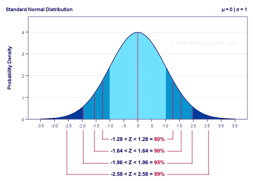
$$Z_{1-^{\alpha}_2} = Z_{.975} \approx 1.96$$

The figure below illustrates these and some other critical z-values for different \(\alpha\) levels. The exact values can easily be looked up in Excel or Googlesheets as shown in Normal Distribution - Quick Tutorial.

For our example, the 95% confidence interval is

$$CI_{\delta} = -.048 - .0473 \cdot 1.96 \lt \delta \lt -.048 + .0473 \cdot 1.96 =$$

$$CI_{\delta} = -.141 \lt \delta \lt 0.044$$

That is, there's a 95% likelihood that the population difference lies between -.141 and .044. Note that this CI contains zero: a zero difference between the population proportions -meaning that males and females perform equally well- is within a likely range.

Effect Size I - Cohen’s H

Our sample proportions are p1 = 0.72 and p2 = 0.77. Should we consider that a small, medium or large effect? A likely effect size measure is simply the difference between our proportions. However, a more suitable measure is Cohen’s H, defined as $$h = |\;2\cdot arcsin\sqrt{p1} - 2\cdot arcsin\sqrt{p2}\;|$$
where \(arcsin\) refers to the arcsine function.

Basic rules of thumb⁷ are that

• h = 0.2 indicates a small effect;
• h = 0.5 indicates a medium effect;
• h = 0.8 indicates a large effect.

For our example data, Cohen’s H is
$$h = |\;2\cdot arcsin\sqrt{0.72} - 2\cdot arcsin\sqrt{0.77}\;|$$
$$h = |\;2\cdot 1.01 - 2\cdot 1.07\;| = 0.11$$
Our rules of thumb suggest that this effect is close to negligible.

Effect Size II - Phi Coefficient

An alternative effect size measure for the z-test for independent proportions is the phi coefficient, denoted by φ (the Greek letter “phi”). This is simply a Pearson correlation between dichotomous variables.

Following the rules of thumb for correlations⁷, we could propose that

• \(|\;\phi\;| = 0.1\) indicates a small effect;
• \(|\;\phi\;| = 0.3\) indicates a medium effect;
• \(|\;\phi\;| = 0.5\) indicates a large effect.

However, we feel these rules of thumb are clearly disputable: they may be overly strict because | φ | tends to be considerably smaller than | r |.

Z-Tests in Googlesheets

Z-tests were only introduced to SPSS version 27 in 2020. They're completely absent from some other statistical packages such as JASP. We therefore developed this Googlesheet (read-only), partly shown below.

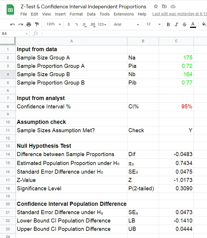
You can download this sheet as Excel and use it as a fast and easy z-test calculator. Given 2 sample proportions and 2 sample sizes, our tool

• checks if the sample size assumption is met;
• computes the 2-tailed-significance-level for the z-test;
• computes a confidence interval for the difference between the proportions;

We prefer this tool over online calculators because

• results in Excel can (and should) be saved with any other project files whereas results from online calculators usually aren't;
• all formulas used in Excel are visible and can thus be verified;
• running many z-tests in Excel can be done effortlessly be expanding the formula section.

SPSS users can readily create the exact right input for the Excel tool with a MEANS command as illustrated by the SPSS syntax below:

Doing so for 2+ dependent variables results in a table as shown below.

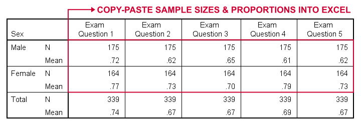
Note that all dependent variables must follow a 0-1 coding in order for this to work.

Relation Z-Test with Other Tests

An alternative for the z-test for independent proportions is a chi-square independence test. The significance level of the latter (which is always 1-tailed) is identical to the 2-tailed significance of the former.

Upon closer inspection, these tests -as well as their assumptions- are statstically equivalent. However, there's 2 reasons for preferring the z-test over the chi-square test:

• the z-test yields a confidence interval for the difference between the proportions;
• running 2 or more z-tests is easier and results in a clearer output table than 2(+) contingency tables with chi-square tests.

Second, the z-test for independent proportions is asymptotically equivalent to the independent samples t-test: their results become more similar insofar as larger sample sizes are used. But -reversely- t-test results for proportions are “off” more insofar as sample sizes are smaller.
Other reasons for preferring the z-test over the t-test are that

• the z-test results in higher power and smaller confidence intervals insofar as smaller sample sizes are used;
• the t-test requires normally distributed dependent variables and equal population-variances whereas the z-test doesn't.

So -in short- use a z-test when appropriate. Your statistical package not including it is a poor excuse for not doing what's right.

Thanks for reading.

References

1. Van den Brink, W.P. & Koele, P. (1998). Statistiek, deel 2 [Statistics, part 2]. Amsterdam: Boom.
2. Van den Brink, W.P. & Koele, P. (2002). Statistiek, deel 3 [Statistics, part 3]. Amsterdam: Boom.
3. Warner, R.M. (2013). Applied Statistics (2nd. Edition). Thousand Oaks, CA: SAGE.
4. Agresti, A. & Franklin, C. (2014). Statistics. The Art & Science of Learning from Data. Essex: Pearson Education Limited.
5. Howell, D.C. (2002). Statistical Methods for Psychology (5th ed.). Pacific Grove CA: Duxbury.
6. Slotboom, A. (1987). Statistiek in woorden [Statistics in words]. Groningen: Wolters-Noordhoff.
7. Cohen, J (1988). Statistical Power Analysis for the Social Sciences (2nd. Edition). Hillsdale, New Jersey, Lawrence Erlbaum Associates.