In statistics, power is the probability of rejecting
a false null hypothesis.
- Power Calculation Example
- Power & Alpha Level
- Power & Effect Size
- Power & Sample Size
- 3 Main Reasons for Power Calculations
- Software for Power Calculations - G*Power
Power - Minimal Example
- In some country, IQ and salary have a population correlation ρ = .10.
- A scientist examines a sample of N = 10 people and finds a sample correlation r = .15.
- He tests the (false) null hypothesis H0 that ρ = 0. The significance level for this test, p = .68.
- Since p > .05, his chosen alpha level, he does not reject his (false) null hypothesis that ρ = 0.
Now, given a sample size of N = 10 and a population correlation ρ = 0.10, what's the probability of correctly rejecting the null hypothesis? This probability is known as power and denoted as (1 - β) in statistics. For the aforementioned example, (1 - β) is only .058 (roughly 6%) as shown below.
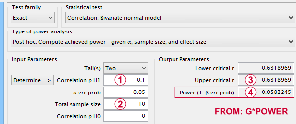
 If a population correlation ρ = .10 and
 we sample N = 10 respondents, then
 we need to find an absolute sample correlation of | r | > .63 for rejecting H0 at α = .05.
 The probability of finding this is only .058.
So even though H0 is false, we're unlikely to actually reject it. Not rejecting a false H0 is known as a committing a type II error.
Type I and Type II Errors
Any null hypothesis may be true or false and we may or may not reject it. This results in the 4 scenarios outlined below.
| Reality: H0 is true | Reality: H0 is false | |
|---|---|---|
| Decision: reject H0 | Type I error Probability = α | Correct decision Probability = (1 - β) = power |
| Decision: retain H0 | Correct decision Probability = (1 - α) | Type II error Probability = β |
As you probably guess, we usually want the power for our tests to be as high as possible. But before taking a look at factors affecting power, let's first try and understand how a power calculation actually works.
Power Calculation Example
A pharmaceutical company wants to demonstrate that their medicine against high blood pressure actually works. They expect the following:
- the average blood pressure in some untreated population is 160 mmHg;
- they expect their medicine to lower this to roughly 154 mmHg;
- the standard deviation should be around 8 mmHg (both populations);
- they plan to use an independent samples t-test at α = 0.05 with N = 20 for either subsample.
Given these considerations, what's the power for this study? Or -alternatively- what's the probability of rejecting H0 that the mean blood pressure is equal between treated and untreated populations?
Obviously, nobody knows the outcomes for this study until it's finished. However, we do know the most likely outcomes: they're our population estimates. So let's for a moment pretend that we'll find exactly these and enter them into a t-test calculator.
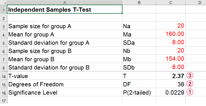 Compute t-test for expected sample sizes, means and SD's in Excel
We expect p = 0.023 so we expect to reject H0.
This is based on a t-distribution with df = 38 degrees of freedom (total sample size N = 40 - 2).
We expect to find t = 2.37 if the population mean difference is 6 mmHg (160 - 154).
Now, this expected (or average) t = 2.37 under the alternative hypothesis Ha is known as a noncentrality parameter or NCP. The NCP tells us how t is distributed under some exact alternative hypothesis and thus allows us to estimate the power for some test. The figure below illustrates how this works.
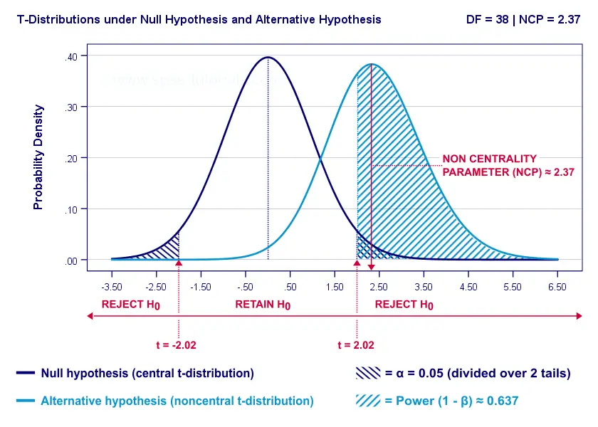
- First off, our H0 is tested using a central t-distribution with df = 38;
- If we test at α = 0.05 (2-tailed), we'll reject H0 if t < -2.02 (left critical value) or if t > 2.02 (right critical value);
- If our alternative hypothesis HA is exactly true, t follows a noncentral t-distribution with df = 38 and NCP = 2.37;
- Under this noncentral t-distribution, the probability of finding t > 2.02 ≈ 0.637. So this is roughly the probability of rejecting H0 -or the power (1 - β)- for our first scenario.
A minor note here is that we'd also reject H0 if t < -2.02 but this probability is almost zero for our first scenario. The exact calculation can be replicated from the SPSS syntax below.
data list free/alpha ncp.
begin data
0.05 2.37
end data.
*Compute left (lct) and right (rct) critical t-values and power.
compute lct = idf.t(0.5 * alpha,38).
compute rct = idf.t(1 - (0.5 * alpha),38).
compute lprob = ncdf.t(lct,38,ncp).
compute rprob = 1 - ncdf.t(rct,38,ncp).
compute power = lprob + rprob.
execute.
*Show 3 decimal places for all values.
formats all (f8.3).
Power and Effect Size
Like we just saw, estimating power requires specifying
- an exact null hypothesis and
- an exact alternative hypothesis.
In the previous example, our scientists had an exact alternative hypothesis because they had very specific ideas regarding population means and standard deviations. In most applied studies, however, we're pretty clueless about such population parameters. This raises the question how do we get an exact alternative hypothesis?
For most tests, the alternative hypothesis can be specified as an effect size measure: a single number combining several means, variances and/or frequencies. Like so, we proceed from requiring a bunch of unknown parameters to a single unknown parameter.
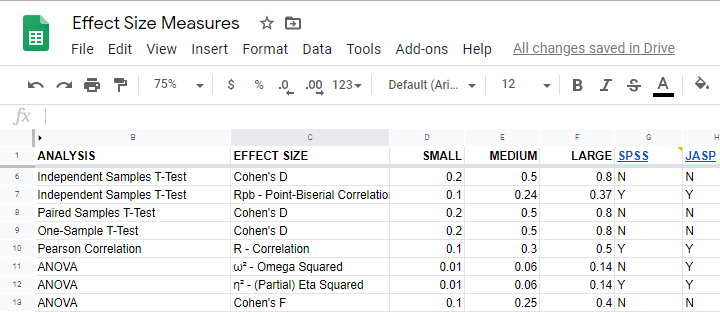
What's even better: widely agreed upon rules of thumb are available for effect size measures. An overview is presented in this Googlesheet, partly shown below.
In applied studies, we often use G*Power for estimating power. The screenshot below replicates our power calculation example for the blood pressure medicine study.
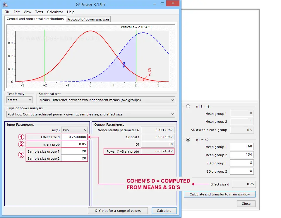 G*Power computes both effect size and power from two means and SD's
Note that estimating power in G*Power only requires
a single estimated effect size measure. Optionally, G*Power computes it for you, given your sample means and SD's.
the alpha level -often 0.05- used for testing the null hypothesis &
one or more sample sizes
Let's now take a look at how these 3 factors relate to power.
Factors Affecting Power
The figure below gives a quick overview how 3 factors relate to power.
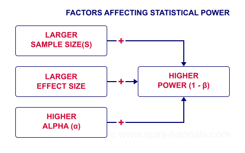
Let's now take a closer look at each of them.
Power & Alpha Level
Everything else equal, increasing alpha increases power. For our example calculation, power increases from 0.637 to 0.753 if we test at α = 0.10 instead of 0.05.
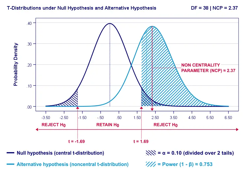
A higher alpha level results in smaller (absolute) critical values: we already reject H0 if t > 1.69 instead of t > 2.02. So the light blue area, indicating (1 - β), increases. We basically require a smaller deviation from H0 for statistical significance.
However, increasing alpha comes at a cost: it increases the probability of committing a type I error (rejecting H0 when it's actually true). Therefore, testing at α > 0.05 is generally frowned upon. In short, increasing alpha basically just decreases one problem by increasing another one.
Power & Effect Size
Everything else equal, a larger effect size results in higher power. For our example, power increases from 0.637 to 0.869 if we believe that Cohen’s D = 1.0 rather than 0.8.
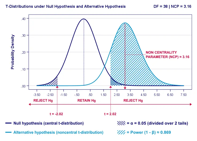
A larger effect size results in a larger noncentrality parameter (NCP). Therefore, the distributions under H0 and HA lie further apart. This increases the light blue area, indicating the power for this test.
Keep in mind, though, that we can estimate but not choose some population effect size. If we overestimate this effect size, we'll overestimate the power for our test accordingly. Therefore, we can't usually increase power by increasing an effect size.
An arguable exception is increasing an effect size by modifying a research design or analysis. For example, (partial) eta squared for a treatment effect in ANOVA may increase by adding a covariate to the analysis.
Power & Sample Size
Everything else equal, larger sample size(s) result in higher power. For our example, increasing the total sample size from N = 40 to N = 80 increases power from 0.637 to 0.912.
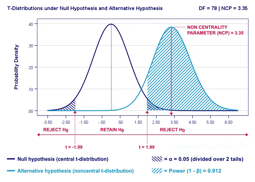
The increase in power stems from our distributions lying further apart. This reflects an increased noncentrality parameter (NCP). But why does the NCP increase with larger sample sizes?
Well, recall that for a t-distribution, the NCP is the expected t-value under HA. Now, t is computed as
$$t = \frac{\overline{X_1} - \overline{X_2}}{SE}$$
where \(SE\) denotes the standard error of the mean difference. In turn, \(SE\) is computed as
$$SE = Sw\sqrt{\frac{1}{n_1} + \frac{1}{n_2}}$$
where \(S_w\) denotes the estimated population SD of the outcome variable. This formula shows that as sample sizes increase, \(SE\) decreases and therefore t (and hence the NCP) increases.
On top of this, degrees of freedom increase (from df = 38 to df = 78 for our example). This results in slightly smaller (absolute) critical t-values but this effect is very modest.
In short, increasing sample size(s) is a sound way to increase the power for some test.
Power & Research Design
Apart from sample size, effect size & α, research design may also affect power. Although there's no exact formulas, some general guidelines are that
- everything else equal, within-subjects designs tend to have more power than between-subjects designs;
- for ANCOVA, including one or two covariates tends to increase power for demonstrating a treatment effect;
- for multiple regression, power for each separate predictor tends to decrease as more predictors are added to the model;
3 Main Reasons for Power Calculations
Power calculations in applied research serve 3 main purposes:
- compute the required sample size prior to data collection. This involves estimating an effect size and choosing α (usually 0.05) and the desired power (1 - B), often 0.80;
- estimate power before collecting data for some planned analyses. This requires specifying the intended sample size, choosing an α and estimating which effect sizes are expected. If the estimated power is low, the planned study may be cancelled or proceed with a larger sample size;
- estimate power after data have been collected and analyzed. This calculation is based on the actual sample size, α used for testing and observed effect size.
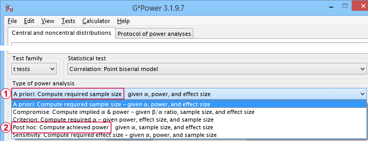 Different types of power analysis are made simple by G*Power
Software for Power Calculations - G*Power
G*Power is freely downloadable software for running the aforementioned and many other power calculations. Among its features are
- computing effect sizes from descriptive statistics (mostly sample means and standard deviations);
- computing power, required sample sizes, required effect sizes and more;
- creating plots that visualize how power, effect size and sample size relate for many different statistical procedures. The figure below shows an example for multiple linear regression.
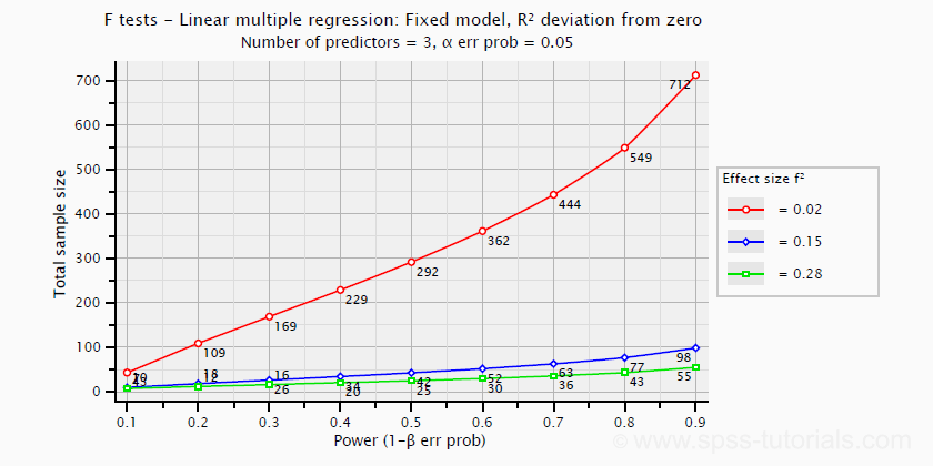 Required sample sizes for multiple linear regression, given desired power,
chosen α and 3 estimated effect sizes
Altogether, we think G*Power is amazing software and we highly recommend using it. The only disadvantage we can think of is that it requires rather unusual effect size measures. Some examples are
- Cohen’s f for ANOVA and
- Cohen’s W for a chi-square test.
This is awkward because the APA and (perhaps therefore) most journal articles typically recommend reporting
- (partial) eta-squared for ANOVA and
- the contingency coefficient or (better) Cramér’s V for a chi-square test.
These are also the measures we typically obtain from statistical packages such as SPSS or JASP. Fortunately, G*Power converts some measures and/or computes them from descriptive statistics like we saw in this screenshot.
Software for Power Calculations - SPSS
In SPSS, observed power can be obtained from the GLM, UNIANOVA and (deprecated) MANOVA procedures. Keep in mind that GLM - short for General Linear Model- is very general indeed: it can be used for a wide variety of analyses including
- (multiple) linear regression;
- t-tests;
- ANCOVA (analysis of covariance);
- repeated measures ANOVA.
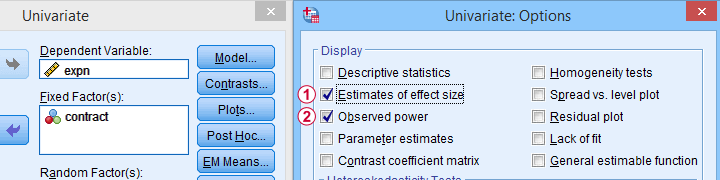 Select Observed power from Analyze - General Linear Model -
Univariate - Options
Other power calculations (required sample sizes or estimating power prior to data collection) were added to SPSS version 27, released in 2020.
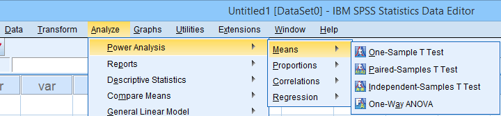 Power Analysis as found in SPSS version 27 onwards
In my opinion, SPSS power analysis is a pathetic attempt to compete with G*Power. If you don't believe me, just try running a couple of power analyses in both programs simultaneously. If you do believe me, ignore SPSS power analysis and just go for G*Power.
Thanks for reading.
THIS TUTORIAL HAS 5 COMMENTS:
By Bogdan on November 17th, 2022
Thanks for the very clear and detailed explanations, they really helped a lot!
By john on November 18th, 2022
At last I've found a very clear description of statistical power. Great explanation. Thanks for this.
By Sabby Grg on May 6th, 2023
Thank you for the clear explanation. I had a few questions about the a priori gpower analysis for the sample size and sensitivity analysis after the data collection. For my project, I initially wanted to run a correlation matrix and then run a multiple linear regression analysis. But the correlation matrix showed that none of the predictors correlated with the outcome variable, so I had to conduct a Spearman’s ranked correlation (data was non-normally distributed). Firstly, should I mention in my report that initially a sample size was determined through f-test power analysis with multiple regression as the statistical test (N=85). But also mention that as there was a change in statistical test, another power analysis was done with t test family and correlation: point biserial model as the statistical test (N=82). As a priori analysis is done before the study, it seemed silly to mention another analysis was done after the study but also doesn’t make sense to just mention the power analysis for multiple regression when I used a correlation test instead.
Secondly, it was recommended to conduct a sensitivity analysis to see what effect size I was powered to detect with my sample size of 81, as I was very close to the required sample size. I did it on G*power with t tests, correlation and sensitivity and the effect size calculation showed a medium effect size, which was what I was aiming for. Even though I didn’t add meet the required sample size, my sample achieved a medium effect size. How should I explain this in my results?
Would the best method be to mention that a power analysis was done with multiple regression as the statistical test, resulting in a sample size of 85. But during data analysis, the correlation matrix showed non-significant relationship between outcome and predictor variables so the appropriate test was Spearman’s rho correlation. A sensitivity analysis showed that even with the sample size of 81, a medium effect size for a correlation test was still achieved (+ justification).
Apologies for the lengthy query. Thank you in advance for your help.
By Ruben Geert van den Berg on May 7th, 2023
Honestly, I'm not buying any of this.
My basic conclusion is that you're just not willing to accept that the effects you're looking for probably aren't there.
For sample sizes of, say, N > 25, Pearson correlations don't require normality. Failing to detect them at N = 81 is pretty clear evidence that some variables just aren't linearly related.
They could still be non linearly related but you should model that via CURVEFIT or non linear transformations rather than going for Spearman correlations.
I'd simply report that the relations you're looking for are probably weak at best. And perhaps use a larger sample size next time.
But blaming lack of power for "non significant" results doesn't strike me as very convincing.
Sorry!
By Sabby Grg on May 7th, 2023
Thank you for your reply. Oh dear, in hindsight, I have worded my query utterly horribly. I think there may have been a misunderstanding, mainly from my lack of knowledge. Firstly, I completely understand your point on the Pearson’s r. I already let my supervisor know that for pre-analysis, I did the Pearson’s correlation before the regression based on the central limit theorem. As there were no significant results from the pre-analysis correlation matrix, it was recommended to do a Spearman’s correlation and justify why (non-normality), instead of regression. Upon reflection, it might be better to use Pearson’s r for the main test since it was already justified through central limit theorem.
Regardless, it was already established that my results are non significant and I had already accepted it. But one of the feedback was to do a sensitivity analysis to check the effect size of my sample of 81. Now, I can see where my initial query seems very misleading because I used the term, justify, when it should have been explain. I thought the recommendation of sensitivity analysis was to explain that my sample size was still powered enough to detect a result but that said result was non-significant. Initially, I wanted to understand how my sample was less than the a priori sample size calculation yet, still was powered to show a medium effect size (indicated by sensitivity analysis). Then after, I was going to explain how the study/sample was powered enough to show a medium effect size but the correlation test showed non-significant results so, it means that there just isn't any relationship between the variables <— This is the part I should’ve added in the initial query and this was my intention. In all honesty, I believe it might be best to leave my sensitivity analysis out if there is such misunderstanding when trying to explain it.
I do apologise for the misunderstanding as trying to justify the non-significant result with power, was not my intention. I was simply trying to understand what explanation there could be for my sample size (81) showing the same effect size as the a priori calculation (85). I know this may all sound amateur from an expert’s point of view but unfortunately, I am at that phase. Even this whole explanation might be flawed but I ask for your consideration.
I will just report inferential statistics using Pearsons’s and leave out the sensitivity analysis. But I do want to thank you for your reply as it has helped me review and reflect.