Cohen’s D is the difference between 2 means
expressed in standard deviations.
- Cohen’s D - Formulas
- Cohen’s D and Power
- Cohen’s D & Point-Biserial Correlation
- Cohen’s D - Interpretation
- Cohen’s D for SPSS Users
Why Do We Need Cohen’s D?
Children from married and divorced parents completed some psychological tests: anxiety, depression and others. For comparing these 2 groups of children, their mean scores were compared using independent samples t-tests. The results are shown below.
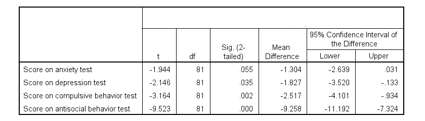
Some basic conclusions are that
- all mean differences are negative. So the second group -children from divorced parents- have higher means on all tests.
- Except for the anxiety test, all differences are statistically significant.
- The mean differences range from -1.3 points to -9.3 points.
However, what we really want to know is are these small, medium or large differences? This is hard to answer for 2 reasons:
- psychological test scores don't have any fixed unit of measurement such as meters, dollars or seconds.
- Statistical significance does not imply practical significance (or reversely). This is because p-values strongly depend on sample sizes.
A solution to both problems is using the standard deviation as a unit of measurement like we do when computing z-scores. And a mean difference expressed in standard deviations -Cohen’s D- is an interpretable effect size measure for t-tests.
Cohen’s D - Formulas
Cohen’s D is computed as
$$D = \frac{M_1 - M_2}{S_p}$$
where
- \(M_1\) and \(M_2\) denote the sample means for groups 1 and 2 and
- \(S_p\) denotes the pooled estimated population standard deviation.
But precisely what is the “pooled estimated population standard deviation”? Well, the independent-samples t-test assumes that the 2 groups we compare have the same population standard deviation. And we estimate it by “pooling” our 2 sample standard deviations with
$$S_p = \sqrt{\frac{(N_1 - 1) \cdot S_1^2 + (N_2 - 1) \cdot S_2^2}{N_1 + N_2 - 2}}$$
Fortunately, we rarely need this formula: SPSS, JASP and Excel readily compute a t-test with Cohen’s D for us.
Cohen’s D in JASP
Running the exact same t-tests in JASP and requesting “effect size” with confidence intervals results in the output shown below.
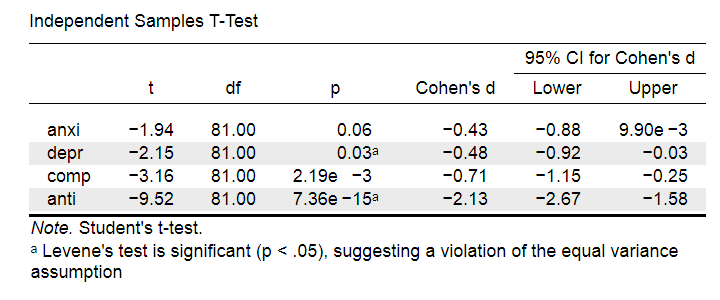
Note that Cohen’s D ranges from -0.43 through -2.13. Some minimal guidelines are that
- d = 0.20 indicates a small effect,
- d = 0.50 indicates a medium effect and
- d = 0.80 indicates a large effect.
And there we have it. Roughly speaking, the effects for
- the anxiety (d = -0.43) and depression tests (d = -0.48) are medium;
- the compulsive behavior test (d = -0.71) is fairly large;
- the antisocial behavior test (d = -2.13) is absolutely huge.
We'll go into the interpretation of Cohen’s D into much more detail later on. Let's first see how Cohen’s D relates to power and the point-biserial correlation, a different effect size measure for a t-test.
Cohen’s D and Power
Very interestingly, the power for a t-test can be computed directly from Cohen’s D. This requires specifying both sample sizes and α, usually 0.05. The illustration below -created with G*Power- shows how power increases with total sample size. It assumes that both samples are equally large.
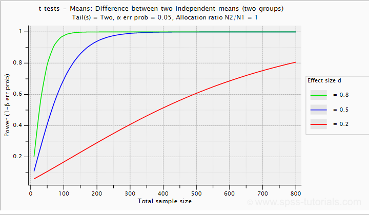
If we test at α = 0.05 and we want power (1 - β) = 0.8 then
- use 2 samples of n = 26 (total N = 52) if we expect d = 0.8 (large effect);
- use 2 samples of n = 64 (total N = 128) if we expect d = 0.5 (medium effect);
- use 2 samples of n = 394 (total N = 788) if we expect d = 0.2 (small effect);
Cohen’s D and Overlapping Distributions
The assumptions for an independent-samples t-test are
- independent observations;
- normality: the outcome variable must be normally distributed in each subpopulation;
- homogeneity: both subpopulations must have equal population standard deviations and -hence- variances.
If assumptions 2 and 3 are perfectly met, then Cohen’s D implies which percentage of the frequency distributions overlap. The example below shows how some male population overlaps with some 69% of some female population when Cohen’s D = 0.8, a large effect.
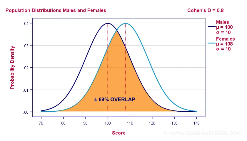
The percentage of overlap increases as Cohen’s D decreases. In this case, the distribution midpoints move towards each other. Some basic benchmarks are included in the interpretation table which we'll present in a minute.
Cohen’s D & Point-Biserial Correlation
An alternative effect size measure for the independent-samples t-test is \(R_{pb}\), the point-biserial correlation. This is simply a Pearson correlation between a quantitative and a dichotomous variable. It can be computed from Cohen’s D with
$$R_{pb} = \frac{D}{\sqrt{D^2 + 4}}$$
For our 3 benchmark values,
- Cohen’s d = 0.2 implies \(R_{pb}\) ± 0.100;
- Cohen’s d = 0.5 implies \(R_{pb}\) ± 0.243;
- Cohen’s d = 0.8 implies \(R_{pb}\) ± 0.371.
Alternatively, compute \(R_{pb}\) from the t-value and its degrees of freedom with
$$R_{pb} = \sqrt{\frac{t^2}{t^2 + df}}$$
Cohen’s D - Interpretation
The table below summarizes the rules of thumb regarding Cohen’s D that we discussed in the previous paragraphs.
| Cohen’s D | Interpretation | Rpb | % overlap | Recommended N |
|---|---|---|---|---|
| d = 0.2 | Small effect | ± 0.100 | ± 92% | 788 |
| d = 0.5 | Medium effect | ± 0.243 | ± 80% | 128 |
| d = 0.8 | Large effect | ± 0.371 | ± 69% | 52 |
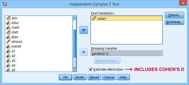
Cohen’s D for SPSS Users
Cohen’s D is available in SPSS versions 27 and higher. It's obtained from
![]()
![]() as shown below.
as shown below.
For more details on the output, please consult SPSS Independent Samples T-Test.
If you're using SPSS version 26 or lower, you can use Cohens-d.xlsx. This Excel sheet recomputes all output for one or many t-tests including Cohen’s D and its confidence interval from
- both sample sizes,
- both sample means and
- both sample standard deviations.
The input for our example data in divorced.sav and a tiny section of the resulting output is shown below.
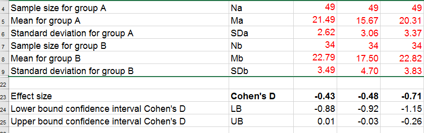
Note that the Excel tool doesn't require the raw data: a handful of descriptive statistics -possibly from a printed article- is sufficient.
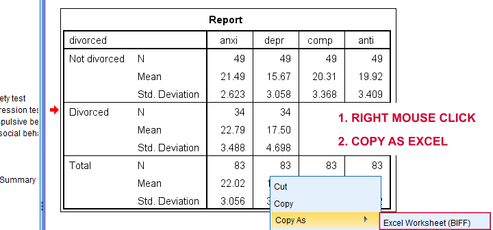
SPSS users can easily create the required input from a simple MEANS command if it includes at least 2 variables. An example is
means anxi to anti by divorced
/cells count mean stddev.
Copy-pasting the SPSS output table as Excel preserves the (hidden) decimals of the results. These can be made visible in Excel and reduce rounding inaccuracies.
Final Notes
I think Cohen’s D is useful but I still prefer R2, the squared (Pearson) correlation between the independent and dependent variable. Note that this is perfectly valid for dichotomous variables and also serves as the fundament for dummy variable regression.
The reason I prefer R2 is that it's in line with other effect size measures: the independent-samples t-test is a special case of ANOVA. And if we run a t-test as an ANOVA, η2 (eta squared) = R2 or the proportion of variance accounted for by the independent variable. This raises the question:
why should we use a different effect size measure
if we compare 2 instead of 3+ subpopulations?
I think we shouldn't.
This line of reasoning also argues against reporting 1-tailed significance for t-tests: if we run a t-test as an ANOVA, the p-value is always the 2-tailed significance for the corresponding t-test. So why should you report a different measure for comparing 2 instead of 3+ means?
But anyway, that'll do for today. If you've any feedback -positive or negative- please drop us a comment below. And last but not least:
thanks for reading!
THIS TUTORIAL HAS 16 COMMENTS:
By Mulugeta Woldeselassie on June 21st, 2025
Fantastic!