A newly updated, ad-free video version of this tutorial
is included in our SPSS beginners course.
- Assumptions
- Independent Samples T-Test Flowchart
- Independent Samples T-Test Dialogs
- Output I - Significance Levels
- Output II - Effect Size
- APA Reporting - Tables & Text
Introduction & Example Data
An independent samples t-test examines if 2 populations
have equal means on some quantitative variable.
For instance, do children from divorced versus non-divorced parents have equal mean scores on psychological tests? We'll walk you through using divorced.sav, part of which is shown below.
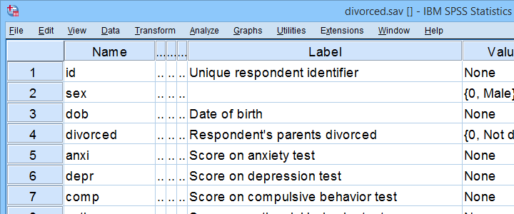
First off, I'd like to shorten some variable labels with the syntax below. Doing so prevents my tables from becoming too wide to fit the pages in my final thesis.
variable labels
anxi 'Anxiety'
depr 'Depression'
comp 'Compulsive Behavior'
anti 'Antisocial Behavior'.
Let's now take a quick look at what's in our data in the first place. Does everything look plausible? Are there any outliers or missing values? I like to find out by running some quick histograms from the syntax below.
frequencies anxi to anti
/format notables
/histogram.
Result
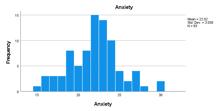
- First, note that all frequency distributions look plausible: we don't see anything weird or unusual.
- Also, none of our histograms show any clear outliers on any of our variables.
- Finally, note that N = 83 for each variable. Since this is our total sample size, this implies that none of them contain any missing values.
After this quick inspection, I like to create a table with sample sizes, means & standard deviations of all dependent variables for both groups separately.
The best way to do so is from
![]()
![]() but the syntax is so simple that just typing it is faster:
but the syntax is so simple that just typing it is faster:
means anxi to anti by divorced
/cells count mean stddev.
Result
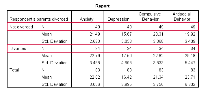
- Note that n = 49 (parents not divorced) and n = 34 (parents divorced) for all dependent variables.
- Also note that children from divorced parents have slightly higher mean scores on most tests. The difference on antisocial behavior (final column) is especially large.
Now, the big question is:
can we conclude from these sample differences
that the entire populations are also different?
An independent samples t-test will answer precisely that. It does, however, require some assumptions.
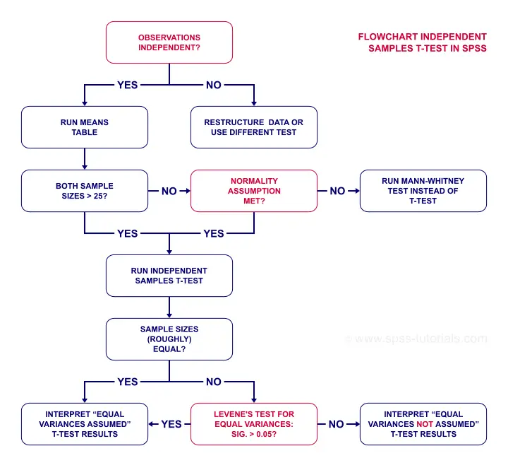
Assumptions
- independent observations. This often holds if each row of data represents a different person.
- Normality: the dependent variable must follow a normal distribution in each subpopulation. This is not needed if both n ≥ 25 or so.
- Homogeneity of variances: both subpopulations must have equal variances on the dependent variable. This is not needed if both sample sizes are roughly equal.
If sample sizes are not roughly equal, then Levene's test may be used to test if homogeneity is met. If that's not the case, then you should report adjusted results. These are shown in the SPSS t-test output under “equal variances not assumed”.
More generally, this procedure is known as the Welch test and also applies to ANOVA as covered in SPSS ANOVA - Levene’s Test “Significant”.
Now, if that's a little too much information, just try and follow the flowchart below.
Independent Samples T-Test Flowchart
Independent Samples T-Test Dialogs
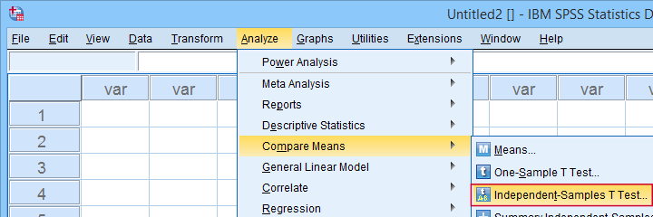
First off, let's navigate to
![]()
![]() as shown below.
as shown below.
Next, we fill out the dialog as shown below.
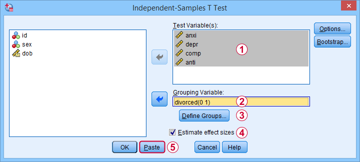
 Sadly, the effect sizes are only available in SPSS version 27 and higher. Since they're very useful, try and upgrade if you're still on SPSS 26 or older.
Anyway, completing these steps results in the syntax below. Let's run it.
T-TEST GROUPS=divorced(0 1)
/MISSING=ANALYSIS
/VARIABLES=anxi depr comp anti
/ES DISPLAY(TRUE)
/CRITERIA=CI(.95).
Output I - Significance Levels
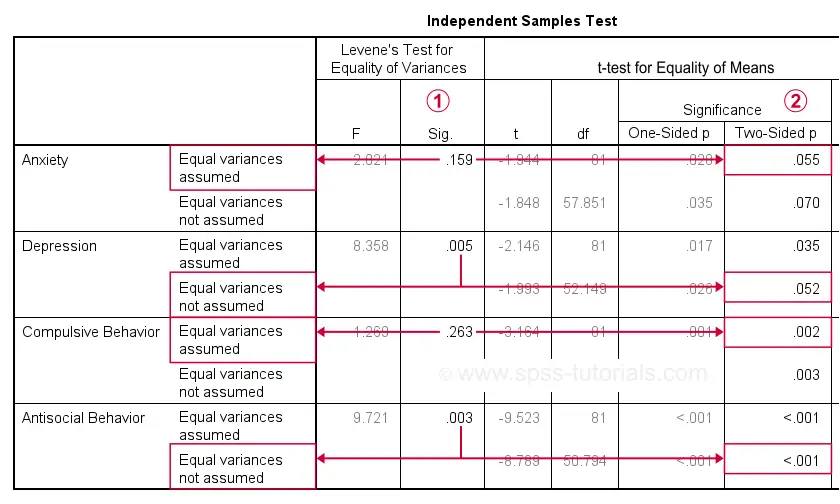
As previously discussed, each dependent variable has 2 lines of results. Which line to report depends on  Levene’s test because our sample sizes are not (roughly) equal:
- if Levene’s test “Sig” or p ≥ .05, then report the “Equal variances assumed”
 t-test results.
 - otherwise, report the “Equal variances not assumed” t-test results.
Following this procedure, we conclude that the mean differences on anxiety (p = .055) and depression (p = .052) are not statistically significant.
The differences on compulsive behavior (p = .002) and antisocial behavior (p < .001), however are both highly “significant”.
This last finding means that our sample differences are highly unlikely if our populations have exactly equal means. The output also includes the mean differences and their confidence intervals.
For example, the mean difference on anxiety is -1.30 points on the anxiety test. But what we don't know, is: should we consider this a small, medium or large difference? We'll answer just that by standardizing our mean differences into effect size measures.
Output II - Effect Size
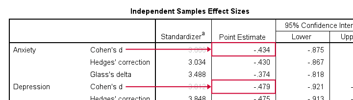
The most common effect size measure for t-tests is Cohen’s D, which we find under “point estimate” in the effect sizes table (only available for SPSS version 27 onwards).
Some general rules of thumb are that
- |d| = 0.20 indicates a small effect;
- |d| = 0.50 indicates a medium effect;
- |d| = 0.80 indicates a large effect.
Like so, we could consider d = -0.43 for our anxiety test roughly a medium effect of divorce and so on.
APA Reporting - Tables & Text
The figure below shows the exact APA style table for reporting the results obtained during this tutorial.
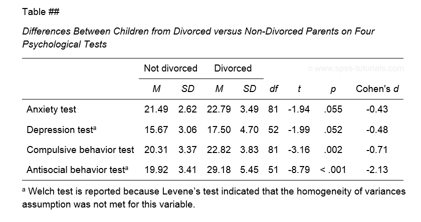
Minor note: if all tests have equal df (degrees of freedom), you may omit this column. In this case, add df to the column header for t as in t(81).
This table was created by combining results from 3 different SPSS output tables in Excel. This doesn't have to be a lot of work if you master a couple of tricks. I hope to cover these in a separate tutorial some time soon.
If you prefer reporting results in text format, follow the example below.
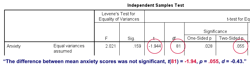
Note that d = -0.43 refers to Cohen’s D here, which is obtained from a separate table as previously discussed.
Final Notes
Most textbooks will tell you to
- use an independent samples t-test for comparing means between 2 subpopulations and
- use ANOVA for comparing means among 3+ subpopulations.
So what happens if we run ANOVA instead of t-tests on the 2 groups in our data? The syntax below does just that.
ONEWAY anxi depr comp anti BY divorced
/ES=OVERALL
/STATISTICS HOMOGENEITY WELCH
/MISSING ANALYSIS
/CRITERIA=CILEVEL(0.95).
Those who ran this syntax will quickly see that most results are identical. This is because an independent samples t-test is a special case of ANOVA. There's 2 important differences, though:
- ANOVA comes up with a single p-value which is identical to p(2-tailed) from the corresponding t-test;
- the effect size for ANOVA is (partial) eta squared rather than Cohen’s D.
This raises an important question:
why do we report different measures for comparing
2 rather than 3+ groups?
My answer: we shouldn't. And this implies that we should
- always report p(2-tailed) for t-tests, never p(1-tailed);
- report eta-squared as the effect size for t-tests and abandon Cohen’s D.
Thanks for reading!
THIS TUTORIAL HAS 79 COMMENTS:
By Barnabas Nehemiah on March 31st, 2024
Very impressive i wish to learn more and have SPSS package install for more practice
By Ruben Geert van den Berg on March 31st, 2024
Hi Barnabas, thanks for the compliment!
If you liked this article, you should definitely subscribe to our YouTube channel as well.
We're going to publish a lot of videos over the coming weeks and they're way better than the (older) written articles.
Thanks!
Ruben
SPSS tutorials
By Abebe on December 21st, 2024
I got a lot from this ,thank you very much
By Samwel Sanga Alananga on May 11th, 2025
An excellent exposition and an example of the T-test for my fellow staff who has been struggling with his PhD. I am sharing with him this link