- Kruskal-Wallis Test Example
- Kruskal-Wallis Test Assumptions
- Kruskal-Wallis Test Formulas
- Kruskal-Wallis Post Hoc Tests
- APA Reporting a Kruskal-Wallis Test
A Kruskal-Wallis test tests if 3(+) populations have
equal mean ranks on some outcome variable.
The figure below illustrates the basic idea.
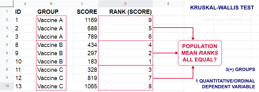
- First off, our scores are ranked ascendingly, regardless of group membership.
- Now, if scores are not related to group membership, then the average mean ranks should be roughly equal over groups.
- If these average mean ranks are very different in our sample, then some groups tend to have higher scores than other groups in our population as well: scores are related to group membership.
Kruskal-Wallis Test - Purposes
The Kruskal-Wallis test is a distribution free alternative for an ANOVA: we basically want to know if 3+ populations have equal means on some variable. However,
- ANOVA is not suitable if the dependent variable is ordinal;
- ANOVA requires the dependent variable to be normally distributed in each subpopulation, especially if sample sizes are small.
The Kruskal-Wallis test is a suitable alternative for ANOVA if sample sizes are small and/or the dependent variable is ordinal.
Kruskal-Wallis Test Example
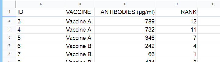
A hospital runs a quick pilot on 3 vaccines: they administer each to N = 5 participants. After a week, they measure the amount of antibodies in the participants’ blood. The data thus obtained are in this Googlesheet, partly shown below.
Now, we'd like to know if some vaccines trigger more antibodies than others in the underlying populations. Since antibodies is a quantitative variable, ANOVA seems the right choice here.
However, ANOVA requires antibodies to be normally distributed in each subpopulation. And due to our minimal sample sizes, we can't rely on the central limit theorem like we usually do (or should anyway). And on top of that,
our sample sizes are too small to examine normality.
Just the emphasize this point, the histograms for antibodies by group are shown below.
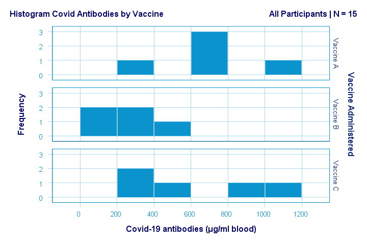
If anything, the bottom two histograms seem slightly positively skewed. This makes sense because the amount of antibodies has a lower bound of zero but no upper bound. However, speculations regarding the population distributions don't get any more serious than that.
A particularly bad idea here is trying to demonstrate normality by running
- a Shapiro-Wilk normality test and/or
- a Kolmogorov-Smirnov test.
Due to our tiny sample sizes, these tests are unlikely to reject the null hypothesis of normality. However, that's merely due to their lack of power and doesn't say anything about the population distributions. Put differently: a different null hypothesis (our variable following a uniform or Poisson distribution) would probably not be rejected either for the exact same data.
In short: ANOVA really requires normality for tiny sample sizes but we don't know if it holds. So we can't trust ANOVA results. And that's why we should use a Kruskal-Wallis test instead.
Kruskal-Wallis Test - Null Hypothesis
The null hypothesis for a Kruskal-Wallis test is that
the mean ranks on some outcome variable
are equal across 3+ populations.
Note that the outcome variable must be ordinal or quantitative in order for “mean ranks” to be meaningful.
Many textbooks propose an incorrect null hypothesis such as:
- some outcome variable has equal medians over 3+ populations or
- some outcome variable follows identical distributions over 3+ populations.
So why are these incorrect? Well, the Kruskal-Wallis formula uses only 2 statistics: ranks sums and the sample sizes on which they're based. It completely ignores everything else about the data -including medians and frequency distributions. Neither of these affect whether the null hypothesis is (not) rejected.
If that still doesn't convince you, we'll perhaps add some example data files to this tutorial. These illustrate that wildly different medians or frequency distributions don't always result in a “significant” Kruskal-Wallis test (or reversely).
Kruskal-Wallis Test Assumptions
A Kruskal-Wallis test requires 3 assumptions1,5,8:
- independent observations;
- the dependent variable must be quantitative or ordinal;
- sufficient sample sizes (say, each ni ≥ 5) unless the exact significance level is computed.
Regarding the last assumption, exact p-values for the Kruskal-Wallis test can be computed. However, this is rarely done because it often requires very heavy computations. Some exact p-values are also found in Use of Ranks in One-Criterion Variance Analysis.
Instead, most software computes approximate (or “asymptotic”) p-values based on the chi-square distribution. This approximation is sufficiently accurate if the sample sizes are large enough. There's no real consensus with regard to required sample sizes: some authors1 propose each ni ≥ 4 while others6 suggest each ni ≥ 6.
Kruskal-Wallis Test Formulas
First off, we rank the values on our dependent variable ascendingly, regardless of group membership. We did just that in this Googlesheet, partly shown below.
Next, we compute the sum over all ranks for each group separately.
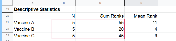
We then enter a) our samples sizes and b) our ranks sums into the following formula:
$$Kruskal\;Wallis\;H = \frac{12}{N(N + 1)}\sum\limits_{i = 1}^k\frac{R_i^2}{n_i} - 3(N + 1)$$
where
- \(N\) denotes the total sample size;
- \(k\) denotes the number of groups we're comparing;
- \(R_i\) denotes the rank sum for group \(i\);
- \(n_i\) denotes the sample size for group \(i\).
For our example, that'll be
$$Kruskal\;Wallis\;H = \frac{12}{15(15 + 1)}(\frac{55^2}{5}+\frac{20^2}{5}+\frac{45^2}{5}) - 3(15 + 1) =$$
$$Kruskal\;Wallis\;H = 0.05\cdot(605 + 80 + 405) - 48 = 6.50$$
\(H\) approximately follows a chi-square (written as χ2) distribution with
$$df = k - 1$$
degrees of freedom (\(df\)) for \(k\) groups. For our example,
$$df = 3 - 1 = 2$$
so our significance level is
$$\chi^2(2) = 6.50, p \approx 0.039.$$
The SPSS output for our example, shown below, confirms our calculations.
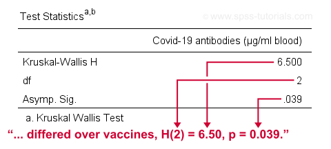
So what do we conclude now? Well, assuming alpha = 0.05, we reject our null hypothesis: the population mean ranks of antibodies are not equal among vaccines. In normal language, our 3 vaccines do not perform equally well. Judging from the mean ranks, it seems vaccine B performs worse than its competitors: its mean rank is lower and this means that it triggered fewer antibodies than the other vaccines.
Kruskal-Wallis Post Hoc Tests
Thus far, we concluded that the amounts of antibodies differ among our 3 vaccines. So precisely which vaccine differs from which vaccine? We'll compare each vaccine to each other vaccine for finding out. This procedure is generally known as running post-hoc tests.
In contrast to popular belief, Kruskal-Wallis post-hoc tests are not equivalent to Bonferroni corrected Mann-Whitney tests. Instead, each possible pair of groups is compared using the following formula:
$$Z_{kw} = \frac{\overline{R}_i - \overline{R}_j}{\sqrt{\frac{N(N + 1)}{12}(\frac{1}{n_i}+\frac{1}{n_j})}}$$
where
- our test statistic, \(Z_{kw}\), approximately follows a standard normal distribution;
- \(\overline R_i\) denotes the mean rank for group \(i\);
- \(N\) denotes the total sample size (including groups not used in this pairwise comparison);
- \(n_i\) denotes the sample size for group \(i\).
For comparing vaccines A and B, that'll be
$$Z_{kw} = \frac{11 - 4}{\sqrt{\frac{15(15 + 1)}{12}(\frac{1}{5}+\frac{1}{5})}} \approx 2.475 $$
$$P(|Z_{kw}| > 2.475) \approx 0.013$$
A Bonferroni correction is usually applied to this p-value because we're running multiple comparisons on (partly) the same observations. The number of pairwise comparisons for \(k\) groups is
$$N_{comp} = \frac{k (k - 1)}{2}$$
Therefore, the Bonferroni corrected p-value for our example is
$$P_{Bonf} = 0.013 \cdot \frac{3 (2 - 1)}{2} \approx 0.040$$
The screenshot from SPSS (below) confirms these findings.
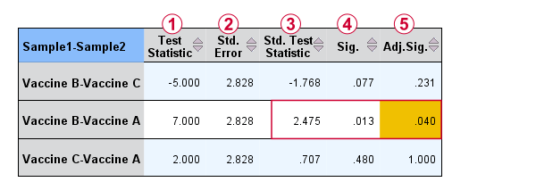
 Oddly, the difference between mean ranks, \(\overline{R}_i - \overline{R}_j\), is denoted as “Test Statistic”.
 The actual test statistic, \(Z_{kw}\) is denoted as “Std. Test Statistic”.
APA Reporting a Kruskal-Wallis Test
For APA reporting our example analysis, we could write something like
“a Kruskal-Wallis test indicated that the amount of antibodies
differed over vaccines, H(2) = 6.50, p = 0.039.
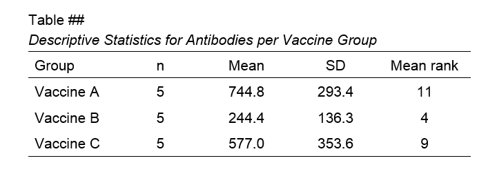
Although the APA doesn't mention it, we encourage reporting the mean ranks and perhaps some other descriptives statistics in a separate table as well.
Right, so that should do. If you've any questions or remarks, please throw me a comment below. Other than that:
Thanks for reading!
References
- Van den Brink, W.P. & Koele, P. (2002). Statistiek, deel 3 [Statistics, part 3]. Amsterdam: Boom.
- Warner, R.M. (2013). Applied Statistics (2nd. Edition). Thousand Oaks, CA: SAGE.
- Agresti, A. & Franklin, C. (2014). Statistics. The Art & Science of Learning from Data. Essex: Pearson Education Limited.
- Field, A. (2013). Discovering Statistics with IBM SPSS Statistics. Newbury Park, CA: Sage.
- Howell, D.C. (2002). Statistical Methods for Psychology (5th ed.). Pacific Grove CA: Duxbury.
- Siegel, S. & Castellan, N.J. (1989). Nonparametric Statistics for the Behavioral Sciences (2nd ed.). Singapore: McGraw-Hill.
- Slotboom, A. (1987). Statistiek in woorden [Statistics in words]. Groningen: Wolters-Noordhoff.
- Kruskal, W.H. & Wallis, W.A. (1952). Use of ranks in one-criterion variance analysis. Journal of the American Statistical Association, 47, 583-621.
THIS TUTORIAL HAS 20 COMMENTS:
By Cristian Herbas on April 26th, 2021
Good work Ruben, now I practice with SPSS for do it applied my dates, I think is work. Many thanks
By Jon Peck on April 26th, 2021
Nice exposition. I wish more people took the K-W route rather than ANOVA. So much ordinal data is wishfully assumed to be scale.
Regarding the post hoc tests, the Bonferroni correction is very conservative, and, especially if the number of groups is large, alternative multiple-testing corrections may be a better choice.
While the KW test in Statistics only offers Bonferroni, the STATS PADJUST extension command, available from the Extension Hub, offers several alternatives. Probably the most popular is Benjamini-Hockberg (also offered in CTABLES). The sig levels can be entered in the syntax (or obtained from a dataset using OMS).
The syntax would be
STATS PADJUST PLIST=.0771 .0133 .4795
METHOD= FDR BONFERRONI.
This gives BH levels of .116, .040, and .480. corresponding to Bonferroni results of
.231, .040, and 1.0
Same conclusions in this case, but the levels are quite different.
By Ruben Geert van den Berg on April 27th, 2021
Hi Jon, that's interesting!
However, I think such corrections can be kinda tricky and should perhaps depend on the type of test you're running. Consider this:
-I use a between-subjects test on 3 groups of n = 10 (so N = 30). Each pairwise comparison uses n = 20 observations so -on average- each observation is used 2 times.
-I then use a within-subjects test on 3 variables using N = 30. In this case, each pairwise comparison uses N = 30 so -on average- each observation is used 3 times.
Intuitively, I'd say that the within-subjects scenario needs a more stringent correction than the between-subjects scenario because it has a less favorable ratio of [actual observations]/[observations used for all pairwise comparisons].
Still, both scenarios would simply yield 3 p-values...
Am I missing something here?
By Jon K Peck on April 27th, 2021
Well, both Bonferroni and Benjamini-Hochberg base the correction on the number of comparisons, but they control the error probabilities differently. Both are based on only the calculated p values and the number of tests. It doesn't matter how the p values were produced. BH controls the proportion of falsely rejected nulls while Bonferroni controls the probability of at least one false rejection.
By Ruben Geert van den Berg on April 28th, 2021
"Both are based on only the calculated p values and the number of tests."
Yes, the syntax you propose
STATS PADJUST PLIST=.0771 .0133 .4795
METHOD= FDR BONFERRONI.
also illustrates this: the raw input is simply a set of p-values. This is the established way to go.
Conceptually, however, it doesn't make sense to me to ignore how many times each independent observation is used on average for some comparison.
For instance, if I compare independent groups a, b, c and d, then the pairwise comparisons a-b and c-d don't have any overlapping observations at all. These 2 comparisons yield 2 p-values but I don't see any reason to adjust these. Nevertheless, they'll add 2 to the number of p-values corrected for (probably 6 for 4 groups).
Even if that's the standard, it doesn't make conceptual sense, does it?