A Pearson correlation is a number between -1 and +1 that indicates
to which extent 2 variables are linearly related.
The Pearson correlation is also known as the “product moment correlation coefficient” (PMCC) or simply “correlation”.
Pearson correlations are only suitable for quantitative variables (including dichotomous variables).
- For ordinal variables, use the Spearman correlation or Kendall’s tau and
- for nominal variables, use Cramér’s V.
Correlation Coefficient - Example
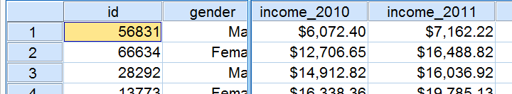
We asked 40 freelancers for their yearly incomes over 2010 through 2014. Part of the raw data are shown below.
Today’s question is:
is there any relation between income over 2010
and income over 2011?
Well, a splendid way for finding out is inspecting a scatterplot for these two variables: we'll represent each freelancer by a dot. The horizontal and vertical positions of each dot indicate a freelancer’s income over 2010 and 2011. The result is shown below.
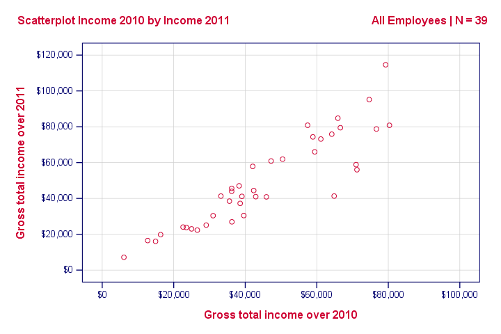
Our scatterplot shows a strong relation between income over 2010 and 2011: freelancers who had a low income over 2010 (leftmost dots) typically had a low income over 2011 as well (lower dots) and vice versa. Furthermore, this relation is roughly linear; the main pattern in the dots is a straight line.
The extent to which our dots lie on a straight line indicates the strength of the relation. The Pearson correlation is a number that indicates the exact strength of this relation.
Correlation Coefficients and Scatterplots
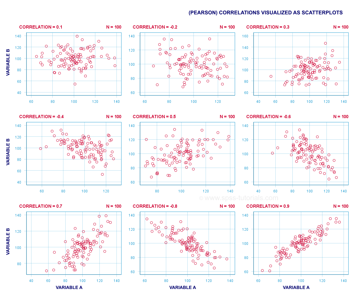
A correlation coefficient indicates the extent to which dots in a scatterplot lie on a straight line. This implies that we can usually estimate correlations pretty accurately from nothing more than scatterplots. The figure below nicely illustrates this point.
Correlation Coefficient - Basics
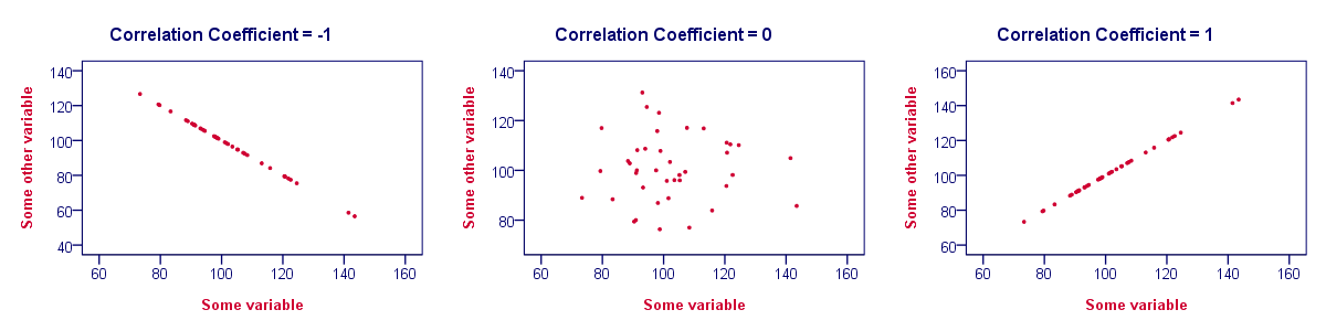
Some basic points regarding correlation coefficients are nicely illustrated by the previous figure. The least you should know is that
- Correlations are never lower than -1. A correlation of -1 indicates that the data points in a scatter plot lie exactly on a straight descending line; the two variables are perfectly negatively linearly related.
- A correlation of 0 means that two variables don't have any linear relation whatsoever. However, some non linear relation may exist between the two variables.
- Correlation coefficients are never higher than 1. A correlation coefficient of 1 means that two variables are perfectly positively linearly related; the dots in a scatter plot lie exactly on a straight ascending line.
Correlation Coefficient - Interpretation Caveats
When interpreting correlations, you should keep some things in mind. An elaborate discussion deserves a separate tutorial but we'll briefly mention two main points.
- Correlations may or may not indicate causal relations. Reversely, causal relations from some variable to another variable may or may not result in a correlation between the two variables.
- Correlations are very sensitive to outliers; a single unusual observation may have a huge impact on a correlation. Such outliers are easily detected by a quick inspection a scatterplot.
Correlation Coefficient - Software
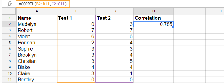
Most spreadsheet editors such as Excel, Google sheets and OpenOffice can compute correlations for you. The illustration below shows an example in Googlesheets.
Correlation Coefficient - Correlation Matrix
Keep in mind that correlations apply to pairs of variables. If you're interested in more than 2 variables, you'll probably want to take a look at the correlations between all different variable pairs. These correlations are usually shown in a square table known as a correlation matrix. Statistical software packages such as SPSS create correlations matrices before you can blink your eyes. An example is shown below.
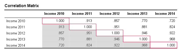
Note that the diagonal elements (in red) are the correlations between each variable and itself. This is why they are always 1.
Also note that the correlations beneath the diagonal (in grey) are redundant because they're identical to the correlations above the diagonal. Technically, we say that this is a symmetrical matrix.
Finally, note that the pattern of correlations makes perfect sense: correlations between yearly incomes become lower insofar as these years lie further apart.
Pearson Correlation - Formula
If we want to inspect correlations, we'll have a computer calculate them for us. You'll rarely (probably never) need the actual formula. However, for the sake of completeness, a Pearson correlation between variables X and Y is calculated by
$$r_{XY} = \frac{\sum_{i=1}^n(X_i - \overline{X})(Y_i - \overline{Y})}{\sqrt{\sum_{i=1}^n(X_i - \overline{X})^2}\sqrt{\sum_{i=1}^n(Y_i - \overline{Y})^2}}$$
The formula basically comes down to dividing the covariance by the product of the standard deviations. Since a coefficient is a number divided by some other number our formula shows why we speak of a correlation coefficient.
Correlation - Statistical Significance
The data we've available are often -but not always- a small sample from a much larger population. If so,
we may find a non zero correlation in our sample
even if it's zero in the population. The figure below illustrates how this could happen.
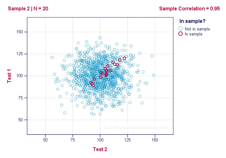
If we ignore the colors for a second, all 1,000 dots in this scatterplot visualize some population. The population correlation -denoted by ρ- is zero between test 1 and test 2.
Now, we could draw a sample of N = 20 from this population for which the correlation r = 0.95.
Reversely, this means that a sample correlation of 0.95 doesn't prove with certainty that there's a non zero correlation in the entire population. However, finding r = 0.95 with N = 20 is extremely unlikely if ρ = 0. But precisely how unlikely? And how do we know?
Correlation - Test Statistic
If ρ -a population correlation- is zero, then the probability for a given sample correlation -its statistical significance- depends on the sample size. We therefore combine the sample size and r into a single number, our test statistic t:
$$T = R\sqrt{\frac{(n - 2)}{(1 - R^2)}}$$
Now, T itself is not interesting. However, we need it for finding the significance level for some correlation. T follows a t distribution with ν = n - 2 degrees of freedom but only if some assumptions are met.
Correlation Test - Assumptions
The statistical significance test for a Pearson correlation requires 3 assumptions:
- independent observations;
- the population correlation, ρ = 0;
- normality: the 2 variables involved are bivariately normally distributed in the population. However, this is not needed for a reasonable sample size -say, N ≥ 20 or so.The reason for this lies in the central limit theorem.
Pearson Correlation - Sampling Distribution
In our example, the sample size N was 20. So if we meet our assumptions, T follows a t-distribution with df = 18 as shown below.
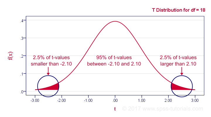
This distribution tells us that there's a 95% probability that -2.1 < t < 2.1, corresponding to -0.44 < r < 0.44. Conclusion:
if N = 20, there's a 95% probability of finding -0.44 < r < 0.44.
There's only a 5% probability of finding a correlation outside this range. That is, such correlations are statistically significant at α = 0.05 or lower: they are (highly) unlikely and thus refute the null hypothesis of a zero population correlation.
Last, our sample correlation of 0.95 has a p-value of 1.55e-10 -one to 6,467,334,654. We can safely conclude there's a non zero correlation in our entire population.
Thanks for reading!
THIS TUTORIAL HAS 32 COMMENTS:
By zahra on July 31st, 2017
you are great! thank you .
By Eugenia on October 12th, 2017
Thank you sososo much!
By Jon Peck on April 25th, 2018
Nice, simple explanation as usual. Might be useful to point out that the point biserial correlation, which people commonly think is necessary with dichotomous variables, is mathematically identical to the Pearson correlation.
By Ruben Geert van den Berg on April 25th, 2018
Thanks for the compliment, Jon! Good suggestion! I should mention the phi coefficient -also a Pearson correlation- as well!
By William Peck on November 1st, 2018
Good presentation, but it's getting a bit complicated in this one.