Simple linear regression is a technique that predicts a metric variable from a linear relation with another metric variable. Remember that “metric variables” refers to variables measured at interval or ratio level. The point here is that calculations -like addition and subtraction- are meaningful on metric variables (“salary” or “length”) but not on categorical variables (“nationality” or “color”).
Example: Predicting Job Performance from IQ
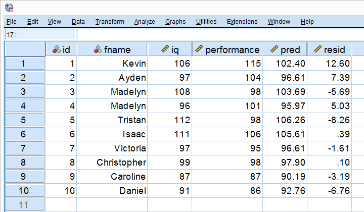
Some company wants to know can we predict job performance from IQ scores? The very first step they should take is to measure both (job) performance and IQ on as many employees as possible. They did so on 10 employees and the results are shown below.
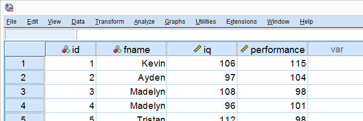
Looking at these data, it seems that employees with higher IQ scores tend to have better job performance scores as well. However, this is difficult to see with even 10 cases -let alone more. The solution to this is creating a scatterplot as shown below.
Scatterplot Performance with IQ
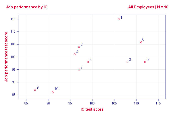
Note that the id values in our data show which dot represents which employee. For instance, the highest point (best performance) is 1 -Kevin, with a performance score of 115.
So anyway, if we move from left to right (lower to higher IQ), our dots tend to lie higher (better performance). That is, our scatterplot shows a positive (Pearson) correlation between IQ and performance.
Pearson Correlation Performance with IQ
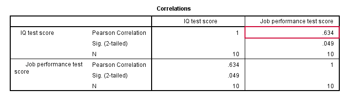
As shown in the previous figure, the correlation is 0.63. Despite our small sample size, it's even statistically significant because p < 0.05. There's a strong linear relation between IQ and performance. But what we haven't answered yet is: how can we predict performance from IQ? We'll do so by assuming that the relation between them is linear. Now the exact relation requires just 2 numbers -and intercept and slope- and regression will compute them for us.
Linear Relation - General Formula
Any linear relation can be defined as Y’ = A + B * X. Let's see what these numbers mean.
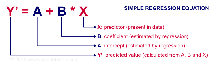
Since X is in our data -in this case, our IQ scores- we can predict performance if we know the intercept (or constant) and the B coefficient. Let's first have SPSS calculate these and then zoom in a bit more on what they mean.
Prediction Formula for Performance
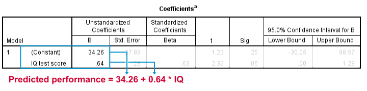
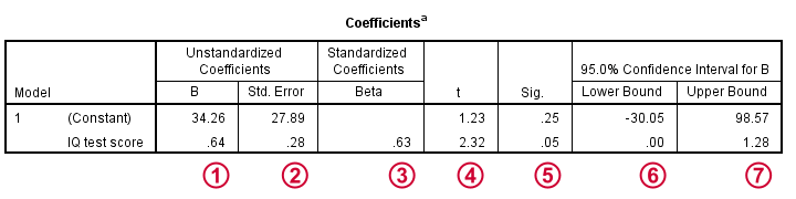
This output tells us that the best possible prediction for job performance given IQ is predicted performance = 34.26 + 0.64 * IQ. So if we get an applicant with an IQ score of 100, our best possible estimate for his performance is predicted performance = 34.26 + 0.64 * 100 = 98.26.
So the core output of our regression analysis are 2 numbers:
- An intercept (constant) of 34.26 and
- a b coefficient of 0.64.
So where did these numbers come from and what do they mean?
B Coefficient - Regression Slope
A b coefficient is number of units increase in Y associated with one unit increase in X. Our b coefficient of 0.64 means that one unit increase in IQ is associated with 0.64 units increase in performance. We visualized this by adding our regression line to our scatterplot as shown below.
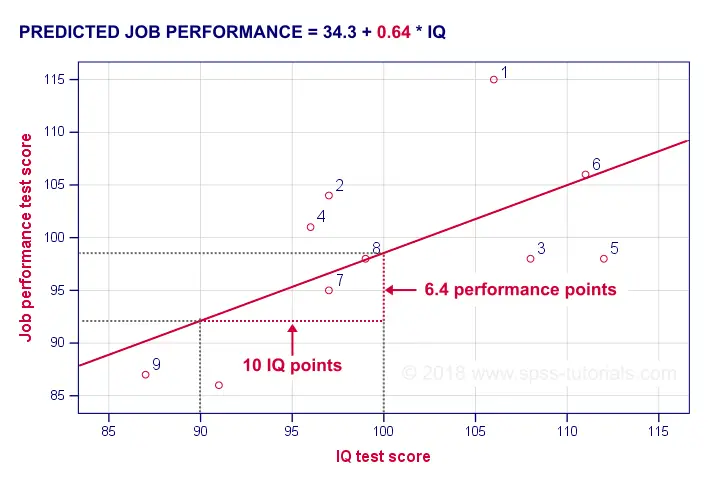
On average, employees with IQ = 100 score 6.4 performance points higher than employees with IQ = 90. The higher our b coefficient, the steeper our regression line. This is why b is sometimes called the regression slope.
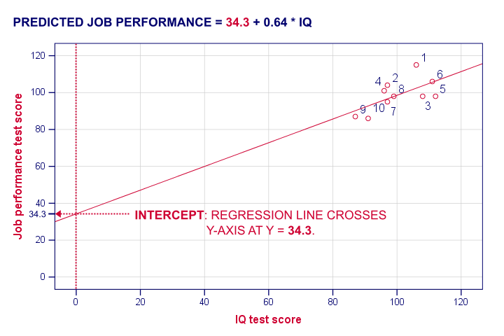
Regression Intercept (“Constant”)
The intercept is the predicted outcome for cases who score 0 on the predictor. If somebody would score IQ = 0, we'd predict a performance of (34.26 + 0.64 * 0 =) 34.26 for this person. Technically, the intercept is the y score where the regression line crosses (“intercepts”) the y-axis as shown below.
I hope this clarifies what the intercept and b coefficient really mean. But why does SPSS come up with a = 34.3 and b = 0.64 instead of some other numbers? One approach to the answer starts with the regression residuals.
Regression Residuals
A regression residual is the observed value - the predicted value on the outcome variable for some case. The figure below visualizes the regression residuals for our example.
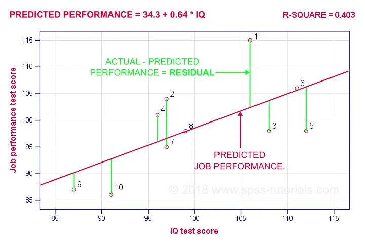
For most employees, their observed performance differs from what our regression analysis predicts. The larger this difference (residual), the worse our model predicts performance for this employee. So how well does our model predict performance for all cases?
Let's first compute the predicted values and residuals for our 10 cases. The screenshot below shows them as 2 new variables in our data. Note that performance = pred + resid.
Our residuals indicate how much our regression equation is off for each case. So how much is our regression equation off for all cases? The average residual seems to answer this question. However, it is always zero: positive and negative residuals simply add up to zero. So instead, we compute the mean squared residual which happens to be the variance of the residuals.
Error Variance
Error variance is the mean squared residual and indicates how badly our regression model predicts some outcome variable. That is, error variance is variance in the outcome variable that regression doesn't “explain”. So is error variance a useful measure? Almost. A problem is that the error variance is not a standardized measure: an outcome variable with a large variance will typically result in a large error variance as well. This problem is solved by dividing the error variance by the variance of the outcome variable. Subtracting this from 1 results in r-square.
R-Square - Predictive Accuracy
R-square is the proportion of variance in the outcome variable that's accounted for by regression. One way to calculate it is from the variance of the outcome variable and the error variance as shown below.
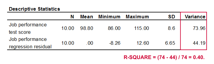
Performance has a variance of 73.96 and our error variance is only 44.19. This means that our regression equation accounts for some 40% of the variance in performance. This number is known as r-square. R-square thus indicates the accuracy of our regression model.
A second way to compute r-square is simply squaring the correlation between the predictor and the outcome variable. In our case, 0.6342 = 0.40. It's called r-square because “r” denotes a sample correlation in statistics.
So why did our regression come up with 34.26 and 0.64 instead of some other numbers? Well, that's because regression calculates the coefficients that maximize r-square. For our data, any other intercept or b coefficient will result in a lower r-square than the 0.40 that our analysis achieved.
Inferential Statistics
Thus far, our regression told us 2 important things:
- how to predict performance from IQ: the regression coefficients;
- how well IQ can predict performance: r-square.
Thus far, both outcomes only apply to our 10 employees. If that's all we're after, then we're done. However, we probably want to generalize our sample results to a (much) larger population. Doing so requires some inferential statistics, the first of which is r-square adjusted.
R-Square Adjusted
R-square adjusted is an unbiased estimator of r-square in the population. Regression computes coefficients that maximize r-square for our data. Applying these to other data -such as the entire population- probably results in a somewhat lower r-square: r-square adjusted. This phenomenon is known as shrinkage.
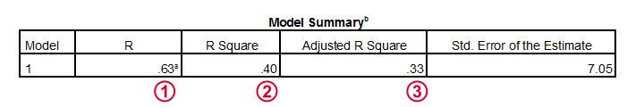
For our data, r-square adjusted is 0.33, which is much lower than our r-square of 0.40. That is, we've quite a lot of shrinkage. Generally,
- smaller sample sizes result in more shrinkage and
- including more predictors (in multiple regression) results in more shrinkage.
Standard Errors and Statistical Significance
Last, let's walk through the last bit of our output.
 The intercept and b coefficient define the linear relation that best predicts the outcome variable from the predictor.
 The standard errors are the standard deviations of our coefficients over (hypothetical) repeated samples. Smaller standard errors indicate more accurate estimates.
 Beta coefficients are standardized b coefficients: b coefficients computed after standardizing all predictors and the outcome variable. They are mostly useful for comparing different predictors in multiple regression. In simple regression, beta = r, the sample correlation.
 t is our test statistic -not interesting but necessary for computing statistical significance.
 “Sig.” denotes the 2-tailed significance for or b coefficient, given the null hypothesis that the population b coefficient is zero.
 The 95% confidence interval gives a likely range for the population b coefficient(s).
Thanks for reading!
THIS TUTORIAL HAS 13 COMMENTS:
By Paison Tazvivinga on June 12th, 2018
This is great.
By Dr. (Prof) Amit Patel on July 27th, 2018
Great Explanation!!!
Thanks
By Ezhumalai G on August 2nd, 2018
I am working as a Statistician / Research consultant in a reputed Medical University in Pondicherry.
Excellent reading material so far what I have studied.
By William Peck on February 28th, 2019
This is very helpful and easy to follow.
By David Stephen A on April 26th, 2019
Very clear and straight forward explanation! Resourceful material!