“Inferential statistics” is the branch of statistics that deals with generalizing outcomes from (small) samples to (much larger) populations. Also, “inferential statistics” is the plural for “inferential statistic”Some key concepts are

• statistical significance testing;
• confidence intervals;
• statistical power;
• null hypotheses;
• standard errors.

All of these basically aim at drawing conclusions (or “inferences”) on populations based on data from samples from those populations.
The basic idea is that sample statistics -such as means, correlations, proportions and many others- may differ from their population counterparts (parameters). However, they do so in a predictable way which tells us how much our sample outcomes are likely to be off.

So How Does It Work?

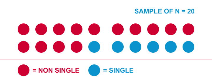
Let me try and explain the basic line of thinking with a simple example. The Hague has roughly 500,000 inhabitants. I’d like to know what percentage of this population is single. Since I can’t ask 500,000 people, I approached 20 of them and asked if they consider themselves single. Like so, I found 6 singles and 14 non singles in my sample of 20. I visualized it below.

A more common way to visualize this result is the frequency distribution shown below. Note that it holds the exact same information as the previous figure.

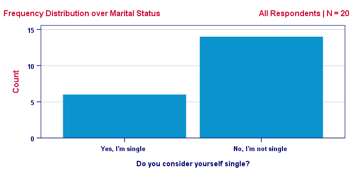
This chart shows how our sample frequencies are distributed (hence “frequency distribution”) over our values: value blue has a frequency of 6, red 14. We could even summarize our outcome as a single number: 30% of our 20 respondents are single.

Are Samples Worthless?

Right, so given my sample of N = 20 and the outcome of 30% singles, what can I conclude -if anything- about my target population, the 500,000 inhabitants of the Hague?

Can I conclude that 30% of the 500,000 inhabitants are single? Or could it be 40% as well? Or 10%? Or 90%? Well, it could actually be basically any percentage. So let's see why.

Imagine I have a vase holding 500k balls, 90% (450k) of which are blue. Now I sample 20 of those balls -completely at random. Could I sample 6 blue and 14 red balls from such a vase? The figure below illustrates the idea.

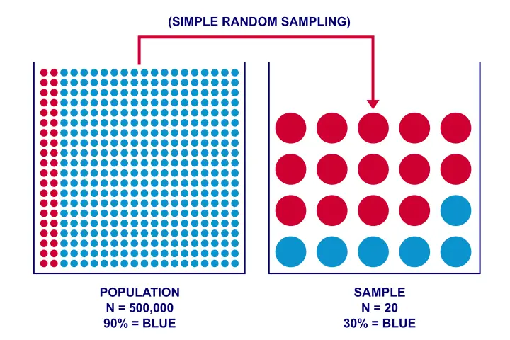
As you can readily see: of course I could sample 6 blue and 14 red balls. My sample of N = 20 balls does not allow me to conclude with certainty that the vase does not contain 90% blue balls.

Now what if my vase contains only 10% blue balls? If I’d sample 20 balls from this vase, could I find 6 blue ones? You’ll probably realize that this is possible indeed.

In short: sampling 6 blue and 14 red balls is possible if 10% or 90% of all balls are blue. It does not rule out either possibility with certainty. So when it comes to concluding anything about my population, a sample is pretty worthless, right?

Wrong.

Thought Experiment: Repeated Sampling

Sure: in theory I could sample 6 blue and 14 red balls from a vase holding 90% blue balls. But it’s practically impossible: the chance is roughly 1 to 4.500,000,000. My small sample basically guarantees that the population percentage is not 90% (but probably much lower).

One way to discover this, is simply trying out the following brute force approach:

• create a fake dataset holding 450k blue and 50k red balls,
• have your computer sample 20 of those 500k balls,
• compute the percentage of blue balls in your sample and

repeat this process 10,000 times. The diagram below visualizes this thought experiment of repeated sampling.

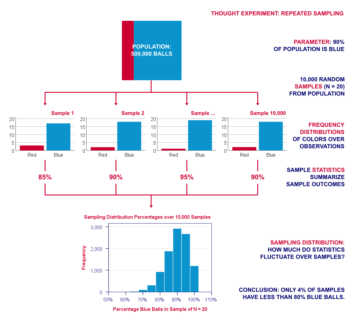
Note that our experiment involves 2 types of frequency distributions. Within each sample, the colors of the balls have a frequency distribution over observations. We can summarize it with a percentage. But here it comes: this percentage -in turn- has a frequency distribution over repeated samples: a sampling distribution.
In a similar vein, correlations, standard deviations and many other statistics also have sampling distributions. And these are useful because they give an idea how much some statistic is likely to be off. This basic reasoning underlies both significance testing and confidence intervals.

So What Does The Sampling Distibution Say?

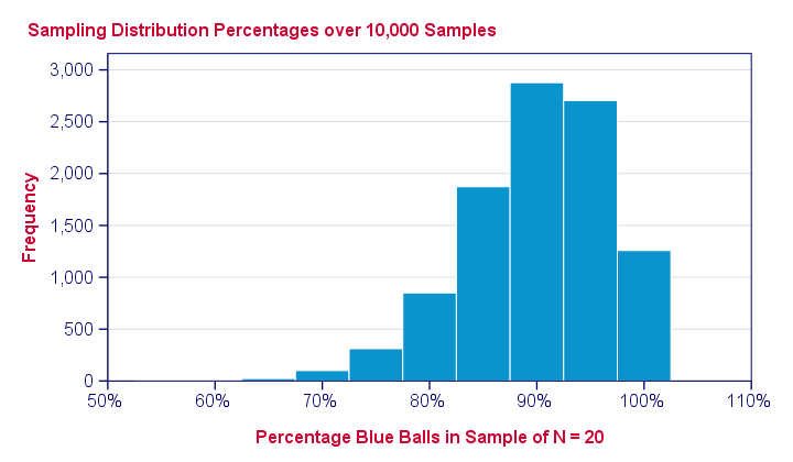
The previous figure shows the sample percentages over 10,000 computerized samples from a population with 90% red balls. So how does that help us? Well, it shows how sample outcomes will fluctuate over samples, given a presumed population percentage.
They don't fluctuate much: the vast majority -some 96%- of sample percentages fall between 80% and 100%. These are likely outcomes; if our population percentage really is 90%, then a sample should probably contain 80% - 100% blue balls. If it doesn't, then the population percentage probably wasn't 90% after all.
So precisely how unlikely are the other outcomes? Well,

• only 4.4% of our 10,000 samples come up with a percentage of 75% or lower;
• only 0.3% come up with 65% or lower;
• the lowest sample percentage is 55% (only 1 sample).

Statistical Significance

As we saw, 4.4% of many samples show 75% or fewer red balls. Another way of saying this is that 1 sample has a 4.4% (or 0.044) probability of holding 75% or fewer. This probability value (p-value) is often called “statistical significance” in statistical tests. Articles often just call it “p” as in “F(2,87) = 3.7, p = .028”. This basically means that 2.8% of many samples should come up with an F-value of 3.7 or larger, given some assumptions (including a null hypothesis).
Now let's try it: we'll feed SPSS a sample of N = 20 cases, 75% of which are blue. And now we'll test the null hypothesis that the population percentage = 90%. The result -shown below- confirms that p -denoted by “Exact Sig. (1-tailed)”- is indeed very close to 0.044.

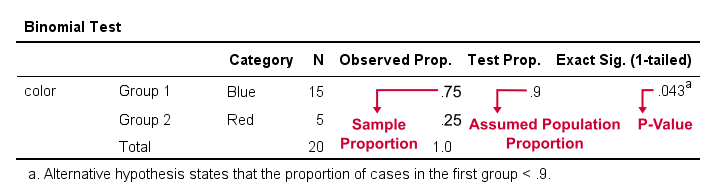
So -again- the p-value of 0.043 means that some 4.3% of many samples should come up with a percentage of 75% or less if the population percentage is 90%. A (rather arbitrary) convention is that we reject the null hypothesis if p < 0.05: if the probability of a sample outcome is less than 5%, then it is so unlikely that we no longer believe that the population percentage is 90%.

Main Sampling Distributions

The sampling distribution we saw -the binomial distribution- isn't used in practice very often. The main sampling distributionsStrictly, these are not sampling distributions but probability density functions. Making this distinction, however, is not necessary for practical purposes. that you will encounter most are

• the (standard) normal distribution;
• the t distribution;
• the F-distribution;
• the chi-square distribution;

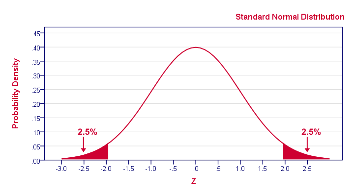
Although it may look different than our binomial distribution, the previous figure conveys the same basic information: some 2.5% of repeated samples should come up with z < -1.96. That is, p(z < -1.96) = 0.025.

Where Can I Get A Sampling Distribution?

Earlier on, we simulated a sampling distribution by having our computer draw 10,000 samples from a dataset containing some population. Although this is a nice and intuitive approach, we don't usually do this. Instead, the sampling distributions for many different statistics -means, correlations, proportions and many others- have been discovered and formulated mathematically. These formulas have been implemented in a lot of software such as MS Excel, OpenOffice and Google Sheets.

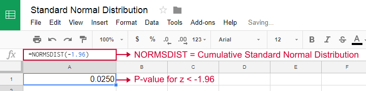
Obviously, all major sampling distributions have also been included in statistical software such as SPSS, Stata and SAS. These packages calculate p-values and confidence intervals straight away for you. So you'll probably skip the sampling distributions altogether in this case.

Final Notes

Right, so inferential statistics basically tries to show how sample outcomes fluctuate over samples. If a statistic fluctuates little, then we can be reasonably confident that it's close to the population parameter that we're after. I hope this quick tutorial gave you a basic idea of how it works.

Thanks for reading!