Introduction & Practice Data File
The Mann-Whitney test is an alternative for the independent samples t-test when the assumptions required by the latter aren't met by the data. The most common scenario is testing a non normally distributed outcome variable in a small sample (say, n < 25).Non normality isn't a serious issue in larger samples due to the central limit theorem.
The Mann-Whitney test is also known as the Wilcoxon test for independent samples -which shouldn't be confused with the Wilcoxon signed-ranks test for related samples.
Research Question
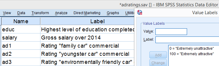
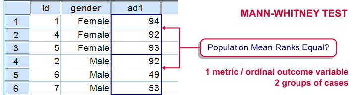
We'll use adratings.sav during this tutorial, a screenshot of which is shown above. These data contain the ratings of 3 car commercials by 18 respondents, balanced over gender and age category. Our research question is whether men and women judge our commercials similarly. For each commercial separately, our null hypothesis is: “the mean ratings of men and women are equal.”
Quick Data Check - Split Histograms
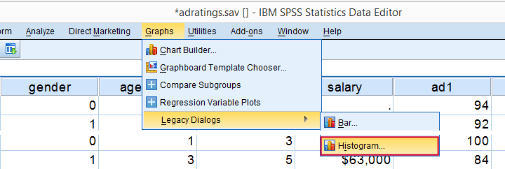
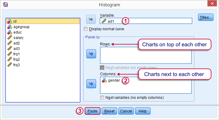
Before running any significance tests, let's first just inspect what our data look like in the first place. A great way for doing so is running some histograms. Since we're interested in differences between male and female respondents, let's split our histograms by gender. The screenshots below guide you through.
Split Histograms - Syntax
Using the menu results in the first block of syntax below. We copy-paste it twice, replace the variable name and run it.
GRAPH
/HISTOGRAM=ad1
/PANEL COLVAR=gender COLOP=CROSS.
GRAPH
/HISTOGRAM=ad2
/PANEL COLVAR=gender COLOP=CROSS.
GRAPH
/HISTOGRAM=ad3
/PANEL COLVAR=gender COLOP=CROSS.
Split Histograms - Results
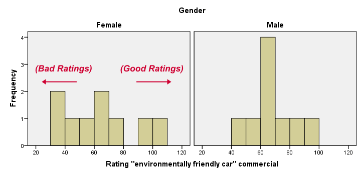
Most importantly, all results look plausible; we don't see any unusual values or patterns. Second, our outcome variables don't seem to be normally distributed and we've a total sample size of only n = 18. This argues against using a t-test for these data.
Finally, by taking a good look at the split histograms, you can already see which commercials are rated more favorably by male versus female respondents. But even if they're rated perfectly similarly by large populations of men and women, we'll still see some differences in small samples. Large sample differences, however, are unlikely if the null hypothesis -equal population means- is really true. We'll now find out if our sample differences are large enough for refuting this hypothesis.
SPSS Mann-Whitney Test - Menu
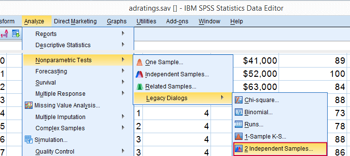
 Depending on your SPSS license, you may or may not have the submenu available. If you don't have it, just skip the step below.
SPSS Mann-Whitney Test - Syntax
Note: selecting results in an extra line of syntax (omitted below).
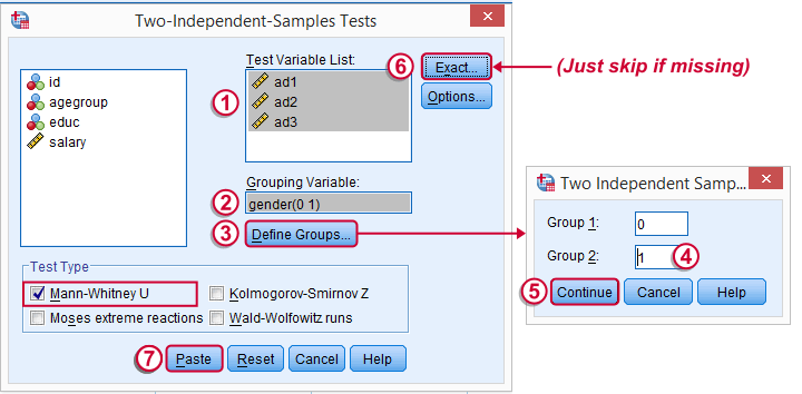
NPAR TESTS
/M-W= ad1 ad2 ad3 BY gender(0 1)
/MISSING ANALYSIS.
SPSS Mann-Whitney Test - Output Descriptive Statistics
The Mann-Whitney test basically replaces all scores with their rank numbers: 1, 2, 3 through 18 for 18 cases. Higher scores get higher rank numbers. If our grouping variable (gender) doesn't affect our ratings, then the mean ranks should be roughly equal for men and women.
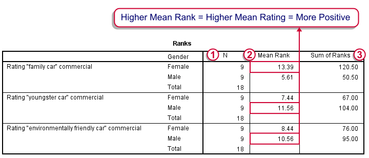
Our first commercial (“Family car”) shows the largest difference in mean ranks between male and female respondents: females seem much more enthusiastic about it. The reverse pattern -but much weaker- is observed for the other two commercials.
SPSS Mann-Whitney Test - Output Significance Tests
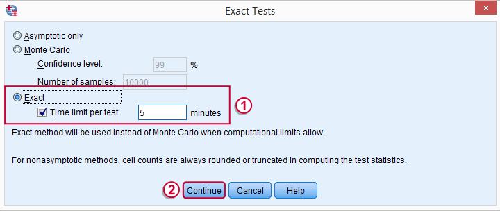
Some of the output shown below may be absent depending on your SPSS license and the sample size: for n = 40 or fewer cases, you'll always get  some exact results.
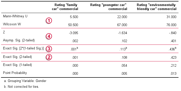
 Mann-Whitney U and Wilcoxon W are our test statistics; they summarize the difference in mean rank numbers in a single number.Note that Wilcoxon W corresponds to the smallest sum of rank numbers from the previous table.
 We prefer reporting Exact Sig. (2-tailed): the exact p-value corrected for ties.
Second best is Exact Sig. [2*(1-tailed Sig.)], the exact p-value but not corrected for ties.
 For larger sample sizes, our test statistics are roughly normally distributed. An approximate (or “Asymptotic”) p-value is based on the standard normal distribution. The z-score and p-value reported by SPSS are calculated without applying the necessary continuity correction, resulting in some (minor) inaccuracy.
SPSS Mann-Whitney Test - Conclusions
Like we just saw, SPSS Mann-Whitney test output may include up to 3 different 2-sided p-values. Fortunately, they all lead to the same conclusion if we follow the convention of rejecting the null hypothesis if p < 0.05: Women rated the “Family Car” commercial more favorably than men (p = 0.001). The other two commercials didn't show a gender difference (p > 0.10). The p-value of 0.001 indicates a probability of 1 in 1,000: if the populations of men and women rate this commercial similarly, then we've a 1 in 1,000 chance of finding the large difference we observe in our sample. Presumably, the populations of men and women don't rate it similarly after all.
So that's about it. Thanks for reading and feel free to leave a comment below!
THIS TUTORIAL HAS 30 COMMENTS:
By Ruben Geert van den Berg on November 11th, 2020
No, I believe all "nonparametric tests" (they're actually distribution free tests) are one-way. Like so, they're either univariate or they include a single between/within subjects factor.
However, keep in mind the central limit theorem: if your sample sizes are reasonably large (like N > 25 or so), you don't generally need the normality assumption for testing means.
Kind regards,
SPSS tutorials
By magdy mahmoud on November 15th, 2020
when U=00 or equal 2 or more what does this means
By Pavol Matula on November 19th, 2020
Excelent,
I apply SW SPSS for education of students (Bc,Mgr)
and for preparing graduation theses
By Ruth Salazar on December 29th, 2020
Thank you, very helpful.
By Faculté Sciences Économiques et Gestion on January 20th, 2026
Thank you for supplying this information.