How do we start analyzing one or many metric variables? My suggestion: first inspect the frequency distributions of all variables separately.
Why? Because metric variables can -and do sometimes- have weird values or distributions. We don't want those to end up in newly computed variables or our final results.
A very fast and easy way to get a hold on metric variables is running and inspecting their histograms. We'll do just that on speedtasks.sav, part of which is shown below.

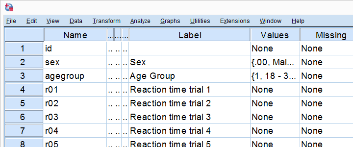Note that no user missing values have been set yet (last column).

SPSS Histograms - The Easy Way

So how do we get our histograms? Well, we can get many in one go from FREQUENCIES. Instead of using SPSS’ menu, copy-paste-edit-running the syntax below is faster and easier.

Results - Case Processing Summary

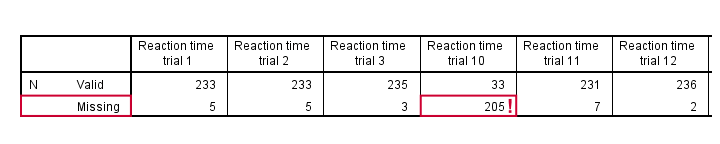
First off, let's take a quick look at the case processing summary in the output viewer window. Note that trial 10 has 205 (!) missing values. Whatever the reason, we shouldn't blindly include it in any multivariate analyses. In fact, we may even exclude it from any analyses.

Results - Histograms

Let's now take a look at the actual histograms. An unfortunate feature -or bug?- is that we don't see any variable names. The output outline shows only variable labels, even after running set ovars both.

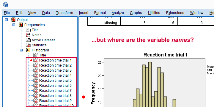
This sucks because we need variable names for setting missing values -if our histograms show any, that is. For the data at hand, the names are pretty straightforward but this is not always the case.

Results - Outliers

Our data hold reaction times and a normal range for them is between some 500 and 2,000 milliseconds -that is, between half a second and 2 seconds. Trial 2 (below) shows some values quite outside this normal range. We could exclude values under 300ms and over 2,500ms by setting them as user missing values.

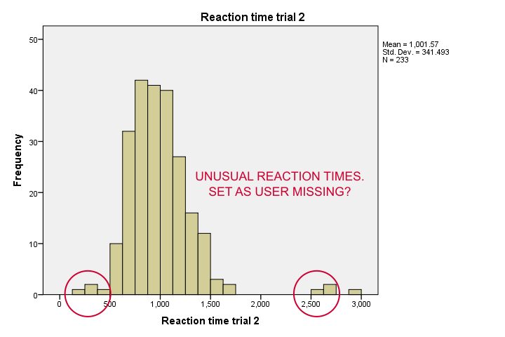
For some very dumb reason, SPSS does not allow setting 2 ranges of missing values (below 300ms and 2,500ms and over). A solution -ugly but often necessary- is to RECODE all values below 300ms and below into 250 and set that as missing.
Strictly, this is unsound practice because we're discarding part of the information in our data. If that's a real concern, try the SPSS Clone Variables Tool.

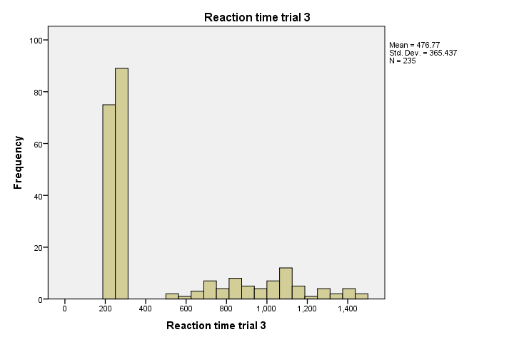
Results - Weird Distribution

Next, note that trial 3 has a seriously weird distribution with huge peaks between 200ms and 300ms. Whatever the reason for this, we probably want to set these values as missing. Unfortunately, we'll have few valid values left if we do so. So we may want to exclude trial 3 altogether from any analyses.

Results - Another Weird Distribution

Although most of our histograms show plausible distributions, trial 7 looks very odd. It almost seems to give us 2 raised middle fingers. How rude...!

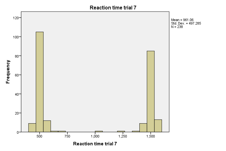
This could be a plausible distribution for some variables such as controversial (“love it or hate it”) statements. For reaction times, however, it's not plausible. Besides, none of the other histograms show this pattern. If all trials were comparable tasks, then perhaps exclude this variable altogether. It seems like something has gone wrong here.
Note that the minimum, maximum, mean and standard deviation all look pretty normal. Simple descriptive statistics would not show anything wrong with this problematic variable.

Final Notes

The data we inspected contain some very nasty surprises. Most data files look way better and many are even problem free. However, I do encounter problematic variables in real data on a very regular basis. The main takeaways from this tutorial are

• inspecting histograms takes very little effort;
• histograms quickly show any problems your metric variables may have;
• descriptive statistics don't always detect all issues;
• choosing which values (or even variables) to exclude can be difficult and disputable.

Thanks for reading!