This tutorial walks through running nice tables and charts for investigating the association between categorical or dichotomous variables. If statistical assumptions are met, these may be followed up by a chi-square test.
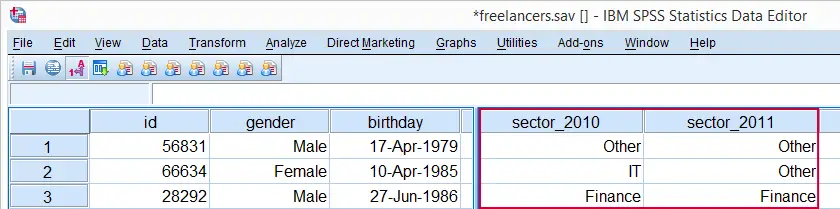
As an example, we'll see whether sector_2010 and sector_2011 in freelancers.sav are associated in any way.
SPSS Quick Data Check
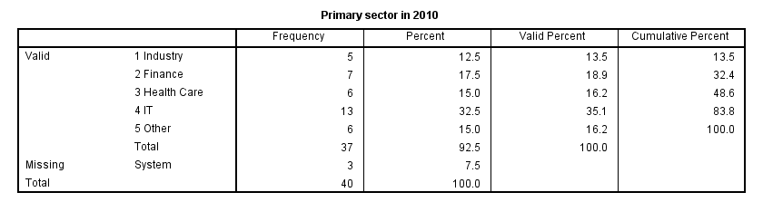
Before doing anything else, let's first just take a quick look at both variables separately. In the syntax below, we first ensure we'll see both values and value labels in our output tables (step 1). Next, we run a basic FREQUENCIES command.
set tnumbers both.
*2. Run frequencies.
frequencies sector_2010 sector_2011.
RECODE System Missing Values
Both variables contain values from 1 through 5 plus system missing values. Since both variables are nominal, we may include these system missings as just another category. This keeps the N nice and constant over analyses and results in cleaner tables.For nicer tables, you may remove “Valid” with a Python script and apply styling with an SPSS table template (.stt file). The syntax below shows how to do so with RECODE.
recode sector_2010 sector_2011 (sysmis = 6).
*2. Explain what formerly missing value means.
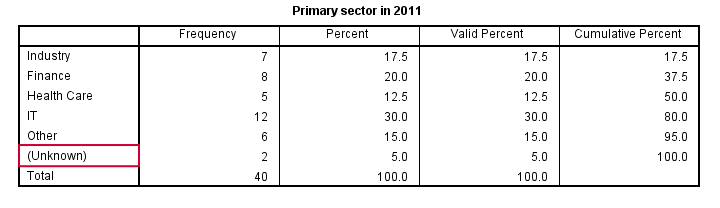
add value labels sector_2010 sector_2011 6 '(Unknown)'.
*3. Show only value labels in output.
set tnumbers labels.
*4. Run clean frequency tables.
frequencies sector_2010 sector_2011.
SPSS CROSSTABS for Both Variables
Thus far, we only had a look at both variables separately. In order to see how they're associated, we'll inspect their contingency table obtained from CROSSTABS. Displaying column percentages without frequencies is our preferred option here.
crosstabs sector_2011 by sector_2010
/cells column.
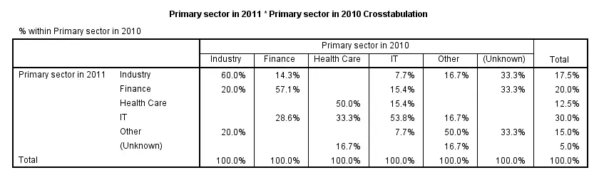
Conclusion: the variables are strongly related.Again, note that we're only describing the data at hand. We're not making any attempt to generalize these results to any larger population. Roughly, most people who worked in a sector in 2010 stayed in the same sector in 2011. For example, 60% of respondents who worked in industry in 2010 stayed in industry. Another 20% moved to finance and the final 20% moved to “other”.
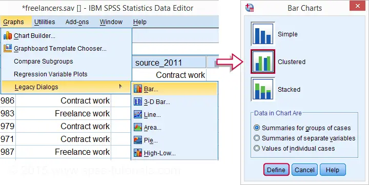
SPSS Clustered Bar Chart Creation
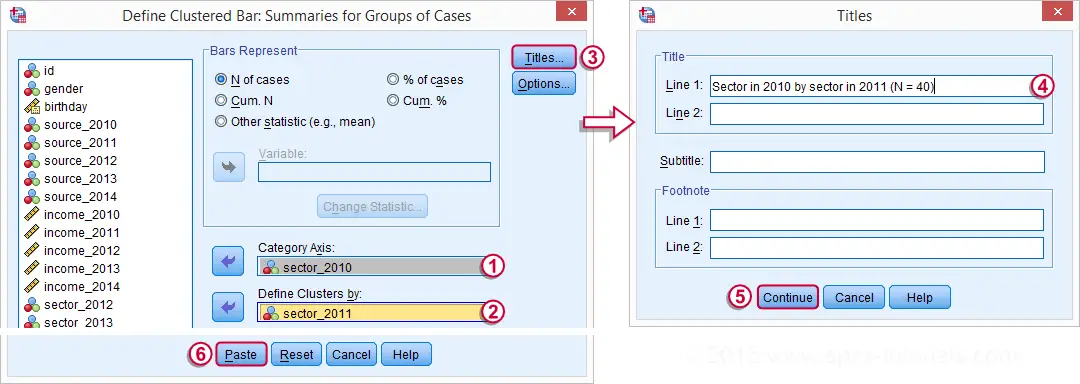
We'll now visualize the contents of the previous table. An option here is a split bar chart but we'll go for a clustered bar chart instead. The screenshots below walk you through the process.
SPSS Clustered Bar Chart Syntax
GRAPH
/BAR(GROUPED)=COUNT BY sector_2011 BY sector_2010
/TITLE='Sector in 2010 by sector in 2011 (N = 40)'.
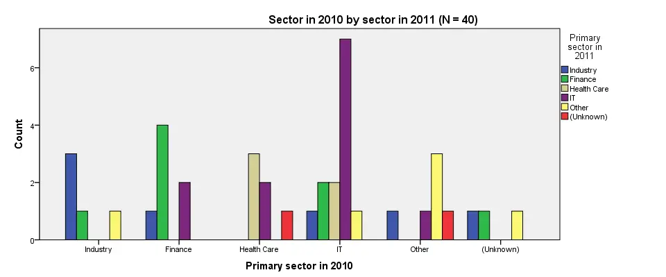
SPSS Clustered Bar Chart Styling
Although our chart is technically correct, it looks appalling. Its default color scheme basically just looks like a bad joke from the software developers. A fast way to prettify this and similar charts is building and applying an SPSS chart template (.sgt file). Our final result after doing so is shown in the last screenshot.
SPSS Clustered Bar Chart Example
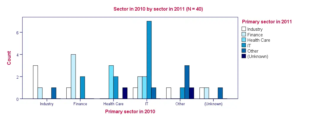
Conclusion: as with the contingency table, we don't see much of a clear pattern here except for people tending to stay in the same sector as the previous year.
THIS TUTORIAL HAS 14 COMMENTS:
By Ruben Geert van den Berg on August 15th, 2018
Hi Salem!
You can download a free 14-day trial version from http://www.ibm.com. After that, you'll have to pay as SPSS isn't free software.
Sorry about that.
By Gbeminiyi Oyinloye on February 7th, 2019
The less we speak about the lack of beauty in SPSS charts the better for the good of humanity.
By Ruben Geert van den Berg on February 7th, 2019
Ha ha! Totally agree! Wise words from a wise man...
However, do read up on SPSS chart templates if you want to create pretty charts fast.
Hope that helps!
SPSS tutorials
By manjari goswami on June 18th, 2023
good