SPSS CROSSTABS – Simple Tutorial & Examples

SPSS CROSSTABS produces contingency tables: frequencies for one variable for each value of another variable separately. If assumptions are met, a chi-square test may follow to test whether an association between the variables is statistically significant. This tutorial, however, aims at quickly walking through the main options for CROSSTABS.
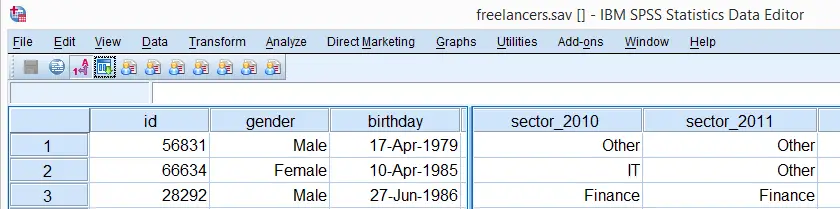
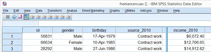
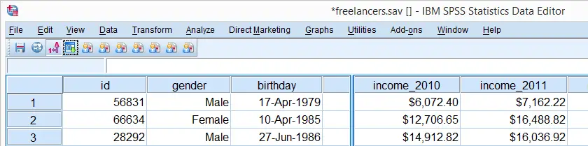
We'll use freelancers.sav throughout this tutorial as a test data file.

SPSS CROSSTABS - Minimal Specification

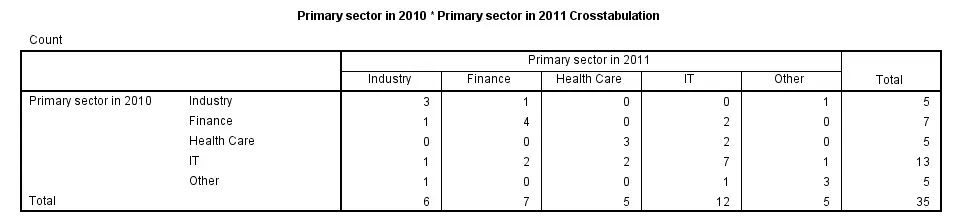
The syntax below demonstrates the simplest possible CROSSTABS command. It generates a table with the frequencies for sector_2010 for each value in sector_2011 separately. The screenshot below shows the result.

SPSS CROSSTABS - CELLS Subcommand

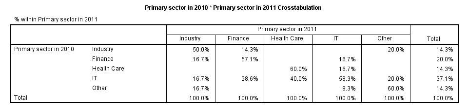
By default, CROSSTABS shows only frequencies (counts). However, the association between variables usually become more visible by displaying row or column percentages. They can be obtained by adding a CELLS subcommand.
Note that multiple cell contents may be chosen simultaneously; the second example below includes both column percentages and frequencies. Specifying ALL on the CELLS subcommand gives a complete overview of the options.

SPSS CROSSTABS - Multiway Tables

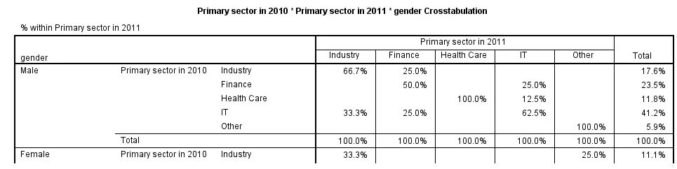
Multiway tables result from including more than one BY clause in CROSSTABS. Like so, the syntax below produces frequencies of sector_2011 for each combination of gender and sector_2010 separately. The following screenshot shows (part of) the result.

SPSS CROSSTABS - Multiple Tables, Similar Columns

Multiple tables with the same column variable but different row variables can be generated by a single CROSSTABS command; simply specify multiple variable names (possibly using TO) before the BY keyword. The syntax below gives an example.

SPSS CROSSTABS - Multiple Tables, Similar Rows

Multiple variables being specified after the BY keyword results in multiple tables with different column variables but the same row variable.

SPSS CROSSTABS - BARCHART Subcommand

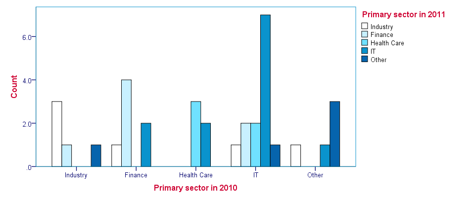
Clustered barcharts can be obtained from CROSSTABS by simply adding a BARCHART subcommand as shown below. However, we prefer to generate such charts via GRAPH because it allows us to set appropriate titles for our charts.
Charts resulting from either option can be styled with an SPSS Chart Template (.sgt) file, which we used for the following screenshot.

SPSS CROSSTABS - STATISTICS Subcommand

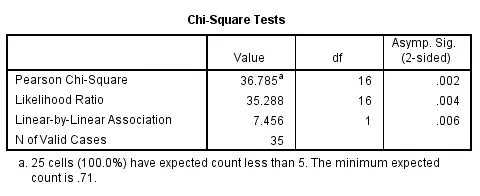
As mentioned in the introduction of this tutorial, CROSSTABS offers a chi-square test for evaluating the statistical significance of an association among the variables involved. It's obtained by specifying CHISQ on the STATISTICS subcommand.
Do keep in mind that SPSS happily produces test results even if their statistical assumptions don't hold, in which case such results may be wildly incorrect.
Besides the chi-square test statistic, many other statistics are available. For a full overview, specify ALL on the STATISTICS subcommand or consult the command syntax reference.

SPSS MEANS – Statistics by Category

SPSS MEANS produces tables containing means and/or other statistics for different groups of cases. These groups are defined by one or more categorical variables. If assumptions are met, MEANS can be followed up by an ANOVA.
This tutorial walks through its main options, pointing out some tips and tricks. You may follow along by downloading and opening freelancers.sav.

SPSS Quick Data Check

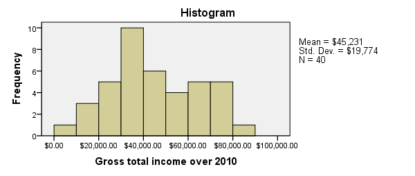
Since we'll run some tables on income_2010, we'll first take a quick look at its histogram by running FREQUENCIES. Note that the second line in the syntax below suppresses frequency tables. We also hide all decimals for income_2010 with FORMATS for suppressing excessive decimals in the output tables.

SPSS MEANS - Minimal Use

Since our histogram doesn't indicate anything unusual, we can now run MEANS. The most simple way to do so is running means income_2010.

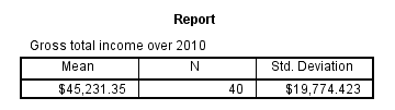
The result is basically the same as DESCRIPTIVES for a single variable but when multiple variables are specified, MEANS will use a different table structure which we'll see later on.

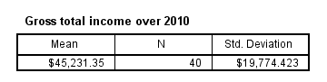
One thing we don't like here is the title (“Report”). However, by using an SPSS Table Template (.stt file), we can make it invisible and enlarge the variable label of the row variable (“Gross total ...”) so it will look like the title. We'll do so throughout the remainder of this tutorial.

SPSS MEANS - Typical Use

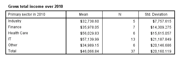
The first MEANS example produced mean incomes over all cases. However, we'll typically use MEANS for generating means for different groups of cases. Like so, the syntax below produces mean incomes for different sectors separately.

SPSS MEANS - CELLS Subcommand

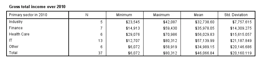
The syntax below has a second line containing a CELLS subcommand. It specifies which statistics (columns) are included in which order.
Note that MEANS has more options here than DESCRIPTIVES, all of which can be included by specifying ALL on the CELLS subcommand.

SPSS MEANS - Multiway Tables

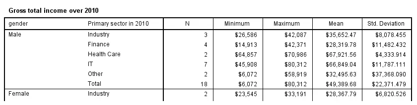
Multiway tables are generated by using more than one BY clause. For example, the syntax below produces mean incomes for each combination of gender and sector separately. You can use even more than two row variables but the resulting table will be rather messy in this case.

SPSS MEANS - Multiple Metric Variables in One Table

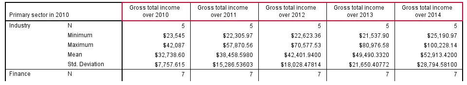
Multiple metric variables may be specified before the BY keyword (possibly using TO) as shown in the syntax below.If you reproduce this table, note that some of the results are wildly incorrect because we failed to specify user missing values for income_2012. This results in one MEANS table with the metric variables as columns.
Statistics and one or more row variables define rows in this case as shown in the following screenshot. If this structure is not to your liking, you may prefer using separate MEANS commands for separate tables instead.

SPSS MEANS - Multiple Tables

Specifying multiple variables after the BY keyword results in multiple tables with the same columns but different (categorical) row variables. The syntax below gives an example.

SPSS MEANS - Final Note

Our discussion of MEANS is by no means exhaustive; you may consult the command syntax reference for more options. We deliberately skipped the STATISTICS subcommand because it doesn't provide any options for evaluating the essential assumptions that underlie statistical significance tests.

SPSS CORRELATIONS – Beginners Tutorial

Also see Pearson Correlations - Quick Introduction.

SPSS CORRELATIONS creates tables with Pearson correlations and their underlying N’s and p-values. For Spearman rank correlations and Kendall’s tau, use NONPAR-CORR. Both commands can be pasted from Analyze Correlate Bivariate.
This tutorial quickly walks through the main options. We'll use freelancers.sav throughout and we encourage you to download it and follow along with the examples.

User Missing Values

Before running any correlations, we'll first specify all values of one million dollars or more as user missing values for income_2010 through income_2014.Inspecting their histograms (also see FREQUENCIES) shows that this is necessary indeed; some extreme values are present in these variables and failing to detect them will have a huge impact on our correlations. We'll do so by running the following line of syntax: missing values income_2010 to income_2014 (1e6 thru hi). Note that “1e6” is a shorthand for a 1 with 6 zeroes, hence one million.

SPSS CORRELATIONS - Basic Use

The syntax below shows the simplest way to run a standard correlation matrix. Note that due to the table structure, all correlations between different variables are shown twice.
By default, SPSS uses pairwise deletion of missing values here; each correlation (between two variables) uses all cases having valid values these two variables. This is why N varies from 38 through 40 in the screenshot below.

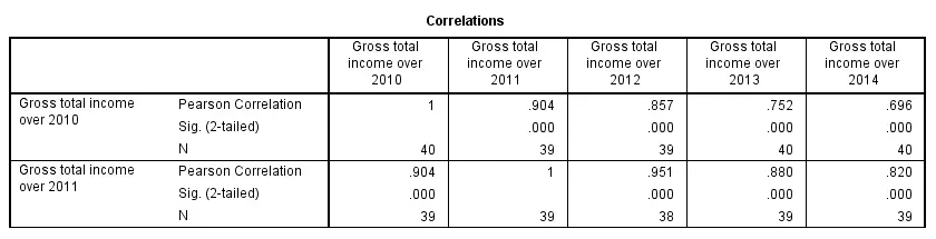
Keep in mind here that p-values are always shown, regardless of whether their underlying statistical assumptions are met or not. Oddly, SPSS CORRELATIONS doesn't offer any way to suppress them. However, SPSS Correlations in APA Format offers a super easy tool for doing so anyway.

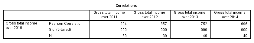
SPSS CORRELATIONS - WITH Keyword

By default, SPSS CORRELATIONS produces full correlation matrices. A little known trick to avoid this is using a WITH clause as demonstrated below. The resulting table is shown in the following screenshot.

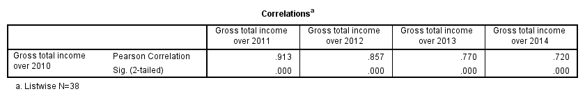
SPSS CORRELATIONS - MISSING Subcommand

Instead of the aforementioned pairwise deletion of missing values, listwise deletion is accomplished by specifying it in a MISSING subcommand.An alternative here is identifying cases with missing values by using NMISS. Next, use FILTER to exclude them from the analysis. Listwise deletion doesn't actually delete anything but excludes from analysis all cases having one or more missing values on any of the variables involved.
Keep in mind that listwise deletion may seriously reduce your sample size if many variables and missing values are involved. Note in the next screenshot that the table structure is slightly altered when listwise deletion is used.

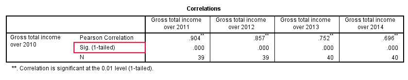
SPSS CORRELATIONS - PRINT Subcommand

By default, SPSS CORRELATIONS shows two-sided p-values. Although frowned upon by many statisticians, one-sided p-values are obtained by specifying ONETAIL on a PRINT subcommand as shown below.
Statistically significant correlations are flagged by specifying NOSIG (no, not SIG) on a PRINT subcommand.

SPSS CORRELATIONS - Notes

More options for SPSS CORRELATIONS are described in the command syntax reference. This tutorial deliberately skipped some of them such as inclusion of user missing values and capturing correlation matrices with the MATRIX subcommand. We did so due to doubts regarding their usefulness.

Thanks for reading!