Mahalanobis Distances in SPSS – A Quick Guide
- Summary
- Mahalanobis Distances - Basic Reasoning
- Mahalanobis Distances - Formula and Properties
- Finding Mahalanobis Distances in SPSS
- Critical Values Table for Mahalanobis Distances
- Mahalanobis Distances & Missing Values
Summary
In SPSS, you can compute (squared) Mahalanobis distances as a new variable in your data file. For doing so, navigate to
![]()
![]() and open the “Save” subdialog as shown below.
and open the “Save” subdialog as shown below.
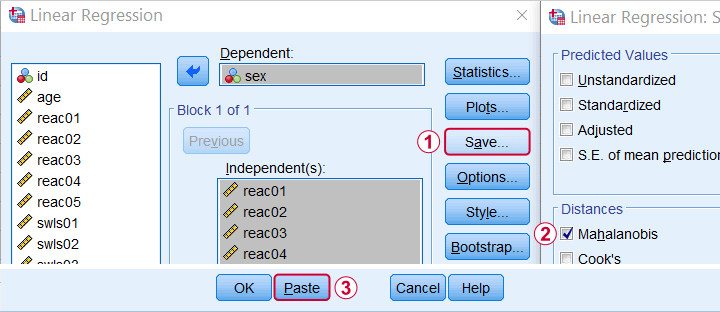
Keep in mind here that Mahalanobis distances are computed only over the independent variables. The dependent variable does not affect them unless it has any missing values. In this case, the situation becomes rather complicated as I'll cover near the end of this article.
Mahalanobis Distances - Basic Reasoning
Before analyzing any data, we first need to know if they're even plausible in the first place. One aspect of doing so is checking for outliers: observations that are substantially different from the other observations. One approach here is to inspect each variable separately and the main options for doing so are
- inspecting histograms;
- inspecting boxplots or
- inspecting z-scores.
Now, when analyzing multiple variables simultaneously, a better alternative is to check for multivariate outliers: combinations of scores on 2(+) variables that are extreme or unusual. Precisely how extreme or unusual a combination of scores is, is usually quantified by their Mahalanobis distance.
The basic idea here is to add up how much each score differs from the mean while taking into account the (Pearson) correlations among the variables. So why is that a good idea? Well, let's first take a look at the scatterplot below, showing 2 positively correlated variables.
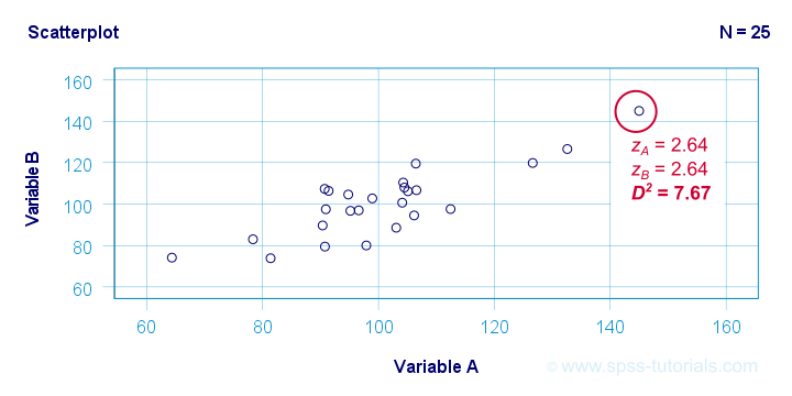
The highlighted observation has rather high z-scores on both variables. However, this makes sense: a positive correlation means that cases scoring high on one variable tend to score high on the other variable too. The (squared) Mahalanobis distance D2 = 7.67 and this is well within a normal range.
So let's now compare this to the second scatterplot shown below.
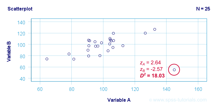
The highlighted observation has a rather high z-score on variable A but a rather low one on variable B. This is highly unusual for variables that are positively correlated. Therefore, this observation is a clear multivariate outlier because its (squared) Mahalanobis distance D2 = 18.03, p < .0005. Two final points on these scatterplots are the following:
- the (univariate) z-scores fail to detect that the highlighted observation in the second scatterplot is highly unusual;
- this observation has a huge impact on the correlation between the variables and is thus an influential data point. Again, this is detected by the (squared) Mahalanobis distance but not by z-scores, histograms or even boxplots.
Mahalanobis Distances - Formula and Properties
Software for applied data analysis (including SPSS) usually computes squared Mahalanobis distances as
\(D^2_i = (\mathbf{x_i} - \mathbf{\overline{x}})'\;\mathbf{S}^{-1}\;(\mathbf{x_i} - \overline{\mathbf{x}})\)
where
- \(D^2\) denotes the squared Mahalanobis distance for case \(i\);
- \(\mathbf{x_i}\) denotes the vector of scores for case \(i\);
- \(\mathbf{\overline{x}}\) denotes the vector of means (centroid) over all cases;
- \(S\) denotes the covariance matrix over all variables.
Some basic properties are that
- Mahalanobis distances can (theoretically) range from zero to infinity;
- Mahalanobis distances are standardized: they are scale independent so they are unaffected by any linear transformations to the variables they're computed on;
- Mahalanobis distances for a single variable are equal to z-scores;
- squared Mahalanobis distances computed over k variables follow a χ2-distribution with df = k under the assumption of multivariate normality.
Finding Mahalanobis Distances in SPSS
In SPSS, you can use the linear regression dialogs to compute squared Mahalanobis distances as a new variable in your data file. For doing so, navigate to
![]()
![]() and open the “Save” subdialog as shown below.
and open the “Save” subdialog as shown below.
Again, Mahalanobis distances are computed only over the independent variables. Although this is in line with most text books, it makes more sense to me to include the dependent variable as well. You could do so by
- adding the actual dependent variable to the independent variables and
- temporarily using an alternative dependent variable that is neither a constant, nor has any missing values.
Finally, if you've any missing values on either the dependent or any of the independent variables, things get rather complicated. I'll discuss the details at the end of this article.
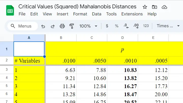
Critical Values Table for Mahalanobis Distances
After computing and inspecting (squared) Mahalanobis distances, you may wonder: how large is too large? Sadly, there's no simple rule of thumb here but most text books suggest that (squared) Mahalanobis distances for which p < .001 are suspicious for reasonable sample sizes. Since p also depends on the number of variables involved, we created a handy overview table in this Googlesheet, partly shown below.
Mahalanobis Distances & Missing Values
Missing values on either the dependent or any of the independent variables may affect Mahalanobis distances. Precisely when and how depends on which option you choose for handling missing values in the linear regression dialogs as shown below.
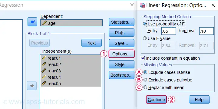
 If you select listwise exclusion,
- Mahalanobis distances are computed for all cases that have zero missing values on the independent variables;
- missing values on the dependent variable may affect the Mahalanobis distances. This is because these are based on the listwise complete covariance matrix over the dependent as well as the independent variables.
 If you select pairwise exclusion,
- Mahalanobis distances are computed for all cases that have zero missing values on the independent variables;
- missing values on the dependent variable do not affect the Mahalanobis distances in any way.
 If you select replace with mean,
- missing values on the dependent and independent variables are replaced with the (variable) means before SPSS proceeds with any further computations;
- Mahalanobis distances are computed for all cases, regardless any missing values;
- \(D^2\) = 0 for cases having missing values on all independent variables. This makes sense because \(\mathbf{x_i} - \mathbf{\overline{x}}\) results in a vector of zeroes after replacing all missing values by means.
References
- Hair, J.F., Black, W.C., Babin, B.J. et al (2006). Multivariate Data Analysis. New Jersey: Pearson Prentice Hall.
- Warner, R.M. (2013). Applied Statistics (2nd. Edition). Thousand Oaks, CA: SAGE.
- Pituch, K.A. & Stevens, J.P. (2016). Applied Multivariate Statistics for the Social Sciences (6th. Edition). New York: Routledge.
- Field, A. (2013). Discovering Statistics with IBM SPSS Statistics. Newbury Park, CA: Sage.
- Howell, D.C. (2002). Statistical Methods for Psychology (5th ed.). Pacific Grove CA: Duxbury.
- Agresti, A. & Franklin, C. (2014). Statistics. The Art & Science of Learning from Data. Essex: Pearson Education Limited.
SPSS – Reorder Variables from Syntax
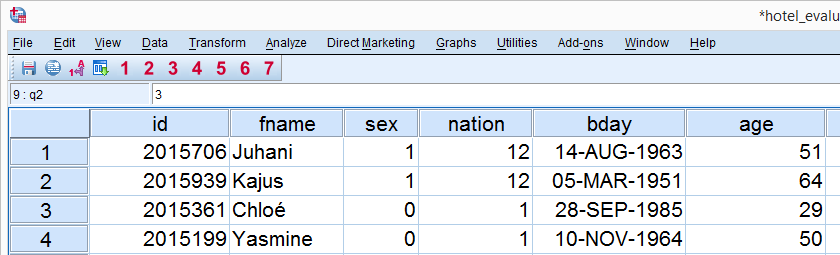
While working in SPSS, it's pretty common to reorder your variables. This tutorial shows how to do so the right way. We encourage you try the examples for yourself by downloading and opening hotel_evaluation.sav, a screenshot of which is shown below.
SPSS Reorder Variables Example 1
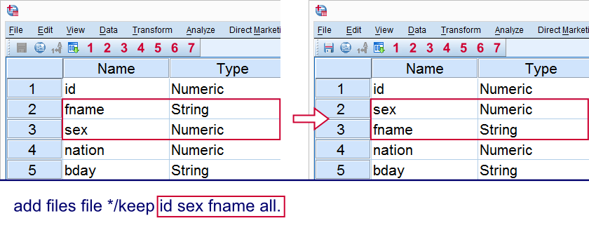
Right, the most common way for reordering variables in SPSS is by running ADD FILES. Before explaining how it works, let's first show that it works in the first place. So suppose we'd like to swap the variables fname and sex. Running the syntax below does just that.
add files file *
/keep id sex fname all.
execute.
Result
How Does It Work?
Remember that ADD FILES merges data sources holding different cases but similar variables. Note that in SPSS syntax, an * addresses the active dataset (often the only data that's open in SPSS).
Now, if we specify this as the only data source, it gets merged with nothing. This means that running
add files file *.
does absolutely nothing whatsoever. However, this command becomes useful if we add a /keep subcommand which tells SPSS which variables to keep (not delete) and in which order.
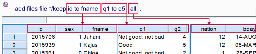
In our first example, we decided to keep id sex fname. Note that the original order here was id fname sex.
Finally, all is a special keyword that addresses all other variables in their original order. Omitting all deletes these variables from our data. The final result of all this is that we basically do nothing except keep all variables in a different order than previously, which is exactly what we were intending.
SPSS Reorder Variables Example 2
Right, we just swapped two variables in our data. But what about moving entire blocks of variables? For instance, suppose we want to have variables q1 through q5 right after fname in our data. Well, this doesn't pose any challenge whatsoever if we use SPSS’ TO keyword. The syntax below shows just how easily it's done.
add files file */keep id to fname q1 to q5 all.
execute.
Result
SPSS Reorder Variables Example 3
Recap: if we're having some data open in SPSS, we can easily reorder our variables by using an ADD FILES command with a keep subcommand.
Is that the only way to get it done? Well, no. If we're done with a dataset, we may use the exact same keep subcommand in a save command as shown below (first example). This is never really necessary but it may save a tiny amount of syntax and processing time.
Just for the sake of completeness, if we know in advance which variables are present in our data, we may also reorder them while opening the data file with get.
SPSS Reorder Variables Syntax Examples
save outfile '10_all_data_prepared.sav'
/keep q1 to q5 all.
*2. Reorder variables when opening data file.
get file 'hotel_evaluation.sav'
/keep q1 to q5 all.
SPSS SORT VARIABLES
There's just one more thing that we need to mention: SPSS (starting from version 16) also has a SORT VARIABLES command. Like so you can sort variables according to variable name, variable type, variable label, format or a couple of other properties.
We obviously needed to mention this command here. However, we very rarely use it in practice. The reason is that the aforementioned sorting options virtually never correspond to the order we desire for our variables. Those who like to give it a quick try anyway, may run something like
sort variables by name.
SPSS Reorder Variables - Final Note
In some cases, you may need to sort your variables in a structured manner that's more complex than covered by this tutorial. An example is sorting (many) variables according to subscripts in their variable names. The way to get such cases done efficiently is by using Python in SPSS.
SPSS Datasets Tutorial 1 – Basics
Introduction
SPSS dataset logic is not always logical. However, for working proficiently with datasets, just a handful of basics is sufficient. These are explained in this tutorial.
This tutorial focuses on working with SPSS datasets. For a definition and some background on datasets, see SPSS Datasets.
Working with SPSS Datasets
- It is recommended you follow along with the steps in this tutorial. You can copy-paste-run the syntax we'll use on idols.sav and service_provider.sav.
- We'll first set our CD to the folder where the files are located. Next, we'll open one of them and compute some test variable.
cd 'd:/downloads'.
get file 'idols.sav'.
Untitled Datasets
 An Untitled Dataset in SPSS
- Note the empty square brackets in the left top corner. These mean that this is an untitled dataset. This is because we haven't assigned a name to it.
- Something specific to an untitled dataset is that it is closed as soon as another dataset is opened. Any changes made to it are discarded.
- For a quick demonstration, run
GET FILE 'service_provider.sav'.. You'll see that the previous dataset has now been replaced by a new (untitled) one.
Named Datasets
- Datasets can be prevented from being closed by naming them with
DATASET NAME. - Dataset names don't need quotes around them and must comply with the naming rules for variables.
get file 'idols.sav'.
dataset name idols_data.
*Open service_provider.sav and apply name to dataset.
get file 'service_provider.sav'.
dataset name service_data.
*Compute test variable.
compute test_0 = 0.
exe.
Now you have two open datasets. The first didn't close upon opening the second because a name ("idols_data") was applied to it.
The Active Dataset
 The Active Dataset in SPSS
- In the previous syntax we also computed a new variable. Upon inspection, you'll see it's present in service_data but not in idols_data.
- This is because service_data was the active dataset when we ran the
COMPUTEcommand. - By default, the active dataset is usually the data you opened or clicked on last. In the windows task bar, the active dataset can be recognized by a red cross in its icon.
- If we want to run syntax on one of the inactive datasets, we'll first activate it. Don't do this by clicking it.
dataset activate idols_data.
compute test_1 = 1.
exe.
Activating idols_data before the COMPUTE command ensures that the new variable will be created in this dataset.
Closing SPSS Datasets
- When we're done with the data we'll close both datasets. (We'll usually first save them as data files. Without doing so, our changes are discarded. This is explained in SPSS Datasets.
- A peculiarity here is that the last open dataset actually stays open. However, its name is removed so it will be gone as soon as other data are opened.
- Alternatively, if you really want it closed, run
NEW FILE.after closing the dataset.
dataset close idols_data.
dataset close service_data.
*Get rid of the last open dataset.
new file.
SPSS Missing Values Functions
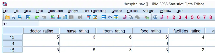
Most real world data contain some (or many) missing values. It's always a good idea to inspect the amount of missingness for avoiding unpleasant surprises later on. In order to do so, SPSS has some missing values functions that are mostly used with COMPUTE, IF AND DO IF. This tutorial demonstrates how to use them effectively. We'll do so by using the last 5 variables in hospital.sav.
Setting User Missing Values
Before discussing SPSS missing values functions, we'll first set 6 as a user missing value for the last 5 variables by running the line of syntax below. missing values doctor_rating to facilities_rating (6).
SPSS Missing Values Functions
| Expression | Meaning | Returns |
|---|---|---|
| MISSING | Evaluate whether value is system missing or user missing | True or false |
| SYSMIS | Evaluate whether value is system missing | True or false |
| NMISS | Return number of missing values over variables | Numeric value |
| NVALID | Return number of valid values over variables | Numeric value |
SPSS MISSING Function
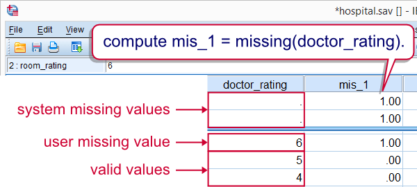
SPSS MISSING function evaluates whether a value is missing (either a user missing value or a system missing value). For example, we'll flag cases that have a missing value on doctor_rating with the syntax below.If the COMPUTE command puzzles you, see Compute A = B = C for an explanation.
compute mis_1 = missing(doctor_rating).
*2. Move flagged cases to top of file.
sort cases mis_1 (d).
SPSS SYSMIS Function
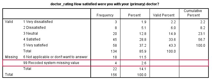
SPSS SYSMIS function evaluates whether a value is system missing. For example, the syntax below uses IF to replace all system missing values by 99. We'll then label it, specify it as user missing and run a quick check with FREQUENCIES.
if sysmis(doctor_rating) doctor_rating = 99.
*2. Add value label 99.
add value labels doctor_rating 99 'Recoded system missing value'.
*3. Specify 6 and 99 as user missings.
missing values doctor_rating (6,99).
*4. Quick check.
frequencies doctor_rating.
SPSS NMISS Function
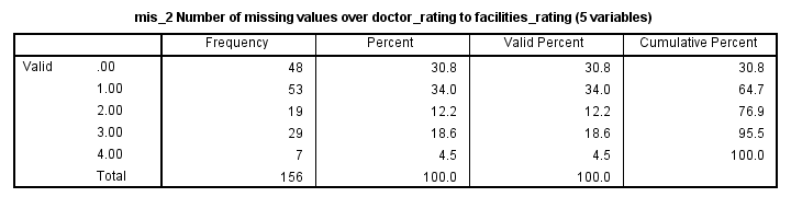
SPSS NMISS function counts missing values within cases over variables. Cases with many missing values may be suspicious and you may want to exclude them from analysis with FILTER or SELECT IF. The syntax runs a quick scan for such cases.
compute mis_2 = nmiss(doctor_rating to facilities_rating).
*2. Apply variable label. Tip: indicate number of variables involved here.
variable labels mis_2 'Number of missing values over doctor_rating to facilities_rating (5 variables)'.
*3. Quick check.
frequencies mis_2.
SPSS NVALID Function
SPSS NVALID function counts the number of valid values over variables. It is equivalent to the number of variables minus NMISS over those variables. Note that the dot operator is a faster alternative for excluding cases from statistical functions (such as MEAN and SUM).
compute valid_1 = nvalid(doctor_rating to facilities_rating).
exe.