SPSS Friedman Test Tutorial

For testing if 3 or more variables have identical population means, our first option is a repeated measures ANOVA. This requires our data to meet some assumptions -like normally distributed variables. If such assumptions aren't met, then our second option is the Friedman test: a nonparametric alternative for a repeated-measures ANOVA.
Strictly, the Friedman test can be used on quantitative or ordinal variables but ties may be an issue in the latter case.

The Friedman Test - How Does it Work?

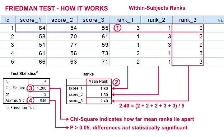
The original variables are ranked within cases.
The mean ranks over cases are computed. If the original variables have similar distributions, then the mean ranks should be roughly equal.
The test-statistic, Chi-Square is like a variance over the mean ranks: it's 0 when the mean ranks are exactly equal and becomes larger as they lie further apart.In ANOVA we find a similar concept: the “mean square between” is basically the variance between sample means. This is explained in ANOVA - What Is It?.
Asymp. Sig. is our p-value. It's the probability of finding our sample differences if the population distributions are equal. The differences in our sample have a large (0.55 or 55%) chance of occurring. They don't contradict our hypothesis of equal population distributions.

The Friedman Test in SPSS

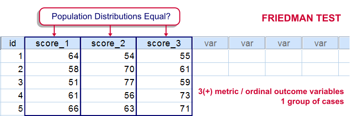
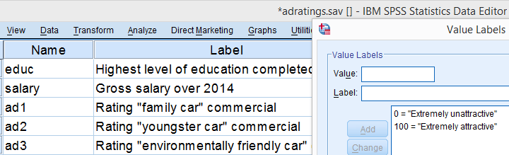
Let's first take a look at our data in adratings.sav, part of which are shown below. The data contain 18 respondents who rated 3 commercials for cars on a percent (0% through 100% attractive) scale.

We'd like to know which commercial performs best in the population. So we'll first see if the mean ratings in our sample are different. If so, the next question is if they're different enough to conclude that the same holds for our population at large. That is, our null hypothesis is that the population distributions of our 3 rating variables are identical.

Quick Data Check

Inspecting the histograms of our rating variables will give us a lot of insight into our data with minimal effort. We'll create them by running the syntax below.

Result

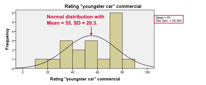
Most importantly, our data look plausible: we don't see any outrageous values or patterns. Note that the mean ratings are pretty different: 83, 55 and 66. Every histogram is based on all 18 cases so there's no missing values to worry about.
Now, by superimposing normal curves over our histograms, we do see that our variables are not quite normally distributed as required for repeated measures ANOVA. This isn't a serious problem for larger sample sizes (say, n > 25 or so) but we've only 18 cases now. We'll therefore play it safe and use a Friedman test instead.

Running a Friedman Test in SPSS

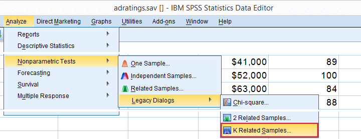
K Related Samples means that we'll compare 3 or more variables measured on the same respondents. This is similar to “within-subjects effect” we find in repeated measures ANOVA.

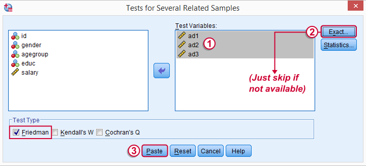
Depending on your SPSS license, you may or may not have the Exact button. If you do, fill it out as below and otherwise just skip it.

SPSS Friedman Test - Syntax

Following these steps results in the syntax below (you'll have 1 extra line if you selected the exact statistics). Let's run it.

SPSS Friedman Test - Output

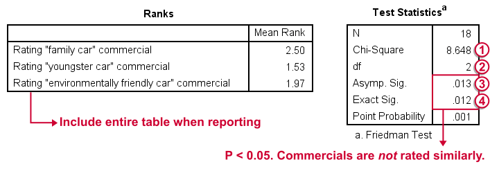
First note that the mean ranks differ quite a lot in favor of the first (“Family Car”) commercial. Unsurprisingly, the mean ranks have the same order as the means we saw in our histogram.
Chi-Square (more correctly referred to as Friedman’s Q) is our test statistic. It basically summarizes how differently our commercials were rated in a single number.
df are the degrees of freedom associated with our test statistic. It's equal to the number of variables we compare - 1. In our example, 3 variables - 1 = 2 degrees of freedom.
Asymp. Sig. is an approximate p-value. Since p < 0.05, we refute the null hypothesis of equal population distributions.“Asymp” is short for “asymptotic”: the more our sample size increases towards infinity, the more the sampling distribution of Friedman’s Q becomes similar to a χ² distribution. Reversely, this χ² approximation is less precise for smaller samples.
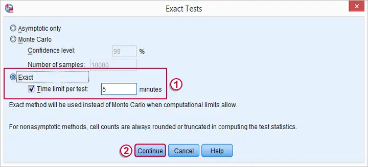
Exact Sig. is the exact p-value. If available, we prefer it over the asymptotic p-value, especially for smaller sample sizes.If there's an exact p-value, then why would anybody ever use an approximate p-value? The basic reason is that the exact p-value requires very heavy computations, especially for larger sample sizes. Modern computers deal with this pretty well but this hasn't always been the case.

Friedman Test - Reporting

As indicated previously, we'll include the entire table of mean ranks in our report. This tells you which commercial was rated best versus worst. Furthermore, we could write something like “a Friedman test indicated that our commercials were rated differently, χ²(2) = 8.65, p = 0.013.“ We personally disagree with this reporting guideline. We feel Friedman’s Q should be called “Friedman’s Q” instead of “χ²”. The latter is merely an approximation that may or may not be involved when calculating the p-value. Furthermore, this approximation becomes less accurate as the sample size decreases. Friedman’s Q is by no means the same thing as χ² so we feel they should not be used interchangeably.

So much for the Friedman test in SPSS. I hope you found this tutorial useful. Thanks for reading.

SPSS Cochran Q Test

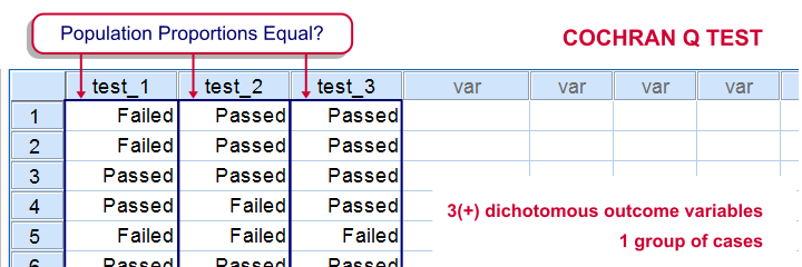
SPSS Cochran Q test is a procedure for testing if the proportions of 3 or more dichotomous variables are equal in some population. These outcome variables have been measured on the same people or other statistical units.

SPSS Cochran Q Test Example

The principal of some university wants to know whether three examns are equally difficult. Fifteen students took these examns and their results are in examn_results.sav.

1. Quick Data Check

It's always a good idea to take a quick look at what the data look like before proceeding to any statistical tests. We'll open the data and inspect some histograms by running FREQUENCIES with the syntax below. Note the TO keyword in step 3.

The histograms indicate that the three variables are indeed dichotomous (there could have been some “Unknown” answer category but it doesn't occur). Since N = 15 for all variables, we conclude there's no missing values. Values 0 and 1 represent “Failed” and “Passed”.We suggest you RECODE your values if this is not the case. We therefore readily see that the proportions of students succeeding range from .53 to .87.

2. Assumptions Cochran Q Test

Cochran's Q test requires only one assumption:

• independent observations (or, more precisely, independent and identically distributed variables);

3. Running SPSS Cochran Q Test

We'll navigate to Analyze Nonparametric Tests Legacy Dialogs K Related Samples...

We move our test variables under Test Variables,
select Descriptive under Statistics,
select Cochran's Q under Test Type and
click Paste
This results in the syntax below which we then run in order to obtain our results.

4. SPSS Cochran Q Test Output

The first table (Descriptive Statistics) presents the descriptives we'll report. Do not report the results from DESCRIPTIVES instead.The reason is that the significance test is (necessarily) based on cases without missing values on any of the test variables. The descriptives obtained from Cochran's test are therefore limited to such complete cases too.
Since N = 15, the descriptives once again confirm that there are no missing values and
the proportions range from .53 to .87.Again, proportions correspond to means if 0 and 1 are used as values.

The table Test Statistics presents the result of the significance test.
The p-value (“Asymp. Sig.”) is .093; if the three tests really are equally difficult in the population, there's still a 9.3% chance of finding the differences we observed in this sample. Since this chance is larger than 5%, we do not reject the null hypothesis that the tests are equally difficult.

5. Reporting Cochran's Q Test Results

When reporting the results from Cochran's Q test, we first present the aforementioned descriptive statistics. Cochran's Q statistic follows a chi-square distribution so we'll report something like “Cochran's Q test did not indicate any differences among the three proportions, χ²(2) = 4.75, p = .093”.