- Confidence Intervals - Example
- Confidence Intervals - How Does it Work?
- Confidence Intervals - Illustration
- Confidence Intervals or Statistical Significance?
- Formulas and Example Calculations
A confidence interval is a range of values
that encloses a parameter with a given likelihood.
So let's say we've a sample of 200 people from a population of 100,000. Our sample data come up with a correlation of 0.41 and indicate that
the 95% confidence interval for this correlation
runs from 0.29 to 0.52.
This means that
- the range of values -0.29 through 0.52-
- has a 95% likelihood
- of enclosing the parameter -the correlation for the entire population- that we'd like to know.
So basically, a confidence interval tells us how much our sample correlation is likely to differ from the population correlation we're after.
Confidence Intervals - Example
El Hierro is the smallest Canary island and has 8,077 inhabitants of 18 years or over. A scientist wants to know their average yearly income. He asks a sample of N = 100. The table below presents his findings.
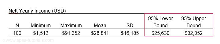
Based on these 100 people, he concludes that the average yearly income for all 8,077 inhabitants is probably between $25,630 and $32,052. So how does that work?
Confidence Intervals - How Does it Work?
Let's say the tax authorities have access to the yearly incomes of all 8,077 inhabitants. The table below shows some descriptive statistics.
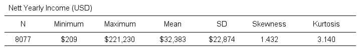
Now, a scientist who samples 100 of these people can compute a sample mean income. This sample mean probably differs somewhat from the $32,383 population mean. Another scientist could also sample 100 people and come up with another different mean. And so on: if we'd draw 100 different samples, we'd probably find 100 different means. In short,
sample means fluctuate over samples.
So how much do they fluctuate? This is expressed by the standard deviation of sample means over samples, known as the standard error -SE- of the mean. SE is calculated as
$$SE = \frac{\sigma}{\sqrt{N}}$$
so for our data that'll be
$$SE = \frac{$22,874}{\sqrt{100}} = $2,287.$$
Right. Now, statisticians also figured out the exact frequency distribution of sample means: the sampling distribution of the mean. For our data, it's shown below.
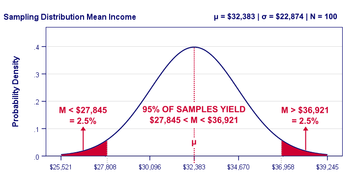
Our graph tells us that 95% of all samples will come up with a mean between roughly $27,808 and $36,958. This is basically the mean ± 2SE:
- the lower bound is roughly $32,383 - 2 · $2,287 = $27,808 and
- the upper bound is roughly $32,383 + 2 · $2,287 = $36,958.
In practice, however, we usually don't know the population mean. So we estimate it from sample data. But how much is a sample mean likely to differ from its population counterpart? Well, we just saw that a sample mean has a 95% probability of falling within ± 2SE of the population mean.
Now, we don't know SE because it depends on the (unknown) population standard deviation. However, we can estimate SE from the sample standard deviation. By doing so, most samples will come up with roughly the correct SE. As a result,
the 95% of samples whose means fall within ± 2SE
typically have confidence intervals enclosing the population mean
as illustrated below.
Confidence Intervals - Illustration
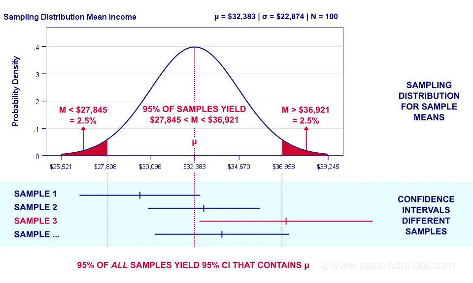 Sampling distribution and confidence intervals. Note that the interval for sample 3 does not contain the population mean μ. This holds for 5% of all CI’s.
Now, a sample having a mean within ±2SE may have a confidence interval not containing the population mean. This may happen if it underestimates the population standard deviation. The reverse may occur too.
However, the sample standard deviation is an unbiased estimator: on average it is exactly correct. So for all samples,
exactly 95% of all 95% confidence intervals
contain the parameter they estimate.
Just as promised.
Confidence Intervals - Basic Properties
Right, so a confidence interval is basically a likely range of values for a parameter such as a population correlation, mean or proportion. Therefore,
wider confidence intervals indicate less precise estimates
for such parameters.
Three factors determine the width of a confidence interval. Everything else equal,
- lower confidence levels result in smaller intervals: 90% CI's are smaller than 95% CI's and these are smaller than 99% CI's. The tradeoff here is that smaller intervals are less likely to contain the parameter we're after: 90% versus 95% or 99%. More precision, less confidence and reversely.
- larger sample sizes result in smaller CI's. However, the width of a CI is linearly related to the square root of the sample size. Therefore, very large samples are inefficient for obtaining precise estimates.
- smaller population SD's result in smaller CI's. However, these are beyond the control of the researcher.
Confidence Intervals or Statistical Significance?
If both are available, confidence intervals. Why? Well, confidence intervals give the same -and more- information than statistical significance. Some examples:
- A 90% confidence interval for the difference between independent means runs from -2.3 to 6.4. Since it contains zero, these means are not significantly different at α 0.90. There's no further need for an independent samples t-test on these data. We already know the outcome.
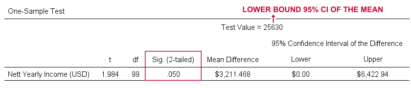
- For our example, the 95% confidence interval ran from $25,630 to $32,052. This renders a one sample t-test useless: we already know that test values in this range result in p > 0.05 and reversely. When testing for the lower or upper bound of the interval, p = 0.05 as SPSS quickly confirms.
So should we stop reporting statistical significance altogether in favor of confidence intervals? Probably not. Confidence intervals are not available for nonparametric tests such as ANOVA or the chi-square independence test. If we compare 2 means, a single confidence interval for the difference tells it all. But that's not going to work for comparing 3 or more means...
Formulas and Example Calculations
Statistical software such as SPSS, Stata or SAS computes confidence intervals for us so there's no need to bother about any formulas or calculations. Do you want to know anyway? Then let's go: we computed the confidence interval for our example in this Googlesheet (downloadable as Excel) as shown below.
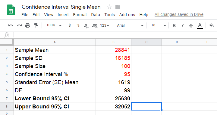
So how does it work? Well, first off, our sample data came up with the descriptive statistics shown below.
We estimate the standard error of the mean as
$$SE_{mean} = \frac{S}{\sqrt{N}}$$
so that'll be
$$SE_{mean} = \frac{$16,185}{\sqrt{100}} = $1,6185.$$
Next,
$$T = \frac{M - \mu}{SE_{mean}}$$
This formula tries to tell you that the difference between the sample mean \(M\) and the population mean \(\mu\) divided by \(SE_{mean}\) follows a t distribution. We're really just standardizing the mean difference here into a z-score (T).
Finally, we need the degrees of freedom given by
$$Df = N - 1$$
so that'll be
$$Df = 100 - 1 = 99.$$
So between which t-values do we find 95% of all (standardized) mean differences? We can look this up in Google sheets as shown below.
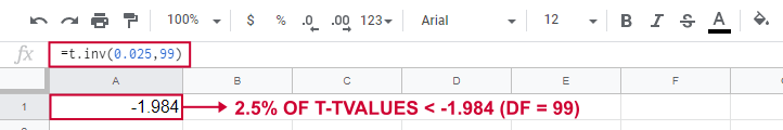
This tells us that a proportion of 0.025 (or 2.5%) of all t-values < -1.984. Because the t-distribution is symmetrical, a proportion of 0.975 of t-values > 1.984. These critical t-values are visualized below.
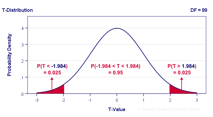
The illustration tells us that our previous rule of thumb of roughly ±2SE is ±1.984SE for this example: 95% of all standardized mean differences are between -1.984 and 1.984. Finally, the 95% confidence interval is
$$M - T_{0.975} \cdot SE_{mean} \lt \mu \lt M + T_{0.975} \cdot SE_{mean} $$
so that'll be
$$$28,841 - 1.984 \cdot $1,619 \lt \mu \lt $28,841 + 1.984 \cdot $1,619$$
which results in
$$$25,630 \lt \mu \lt $32,052.$$
Thanks for reading.
THIS TUTORIAL HAS 14 COMMENTS:
By Syed Suman on July 19th, 2019
Brilliant work! Thank you for this
By Sichilima Faheem on March 9th, 2020
Excellent tutorial. Hats off !!
By Ajibola Bolorunduro on August 21st, 2020
The explanation is comprehensive. I love that
By lusu on September 29th, 2020
when i finished to read it, i found there is a difference with my previous recognize. The difference is about sample having a mean within ±2SE. In China, we use ±3SE.
By Ruben Geert van den Berg on October 1st, 2020
Thanks for your comment!
First off, note that a t-distribution is basically identical to a standard normal distribution if the sample size is reasonable, say N > 25 or so.
For a standard normal distribution, some 4.55% of observations lie outside the mean ±2SE, which is what the 95% confidence interval is based on.
The mean ±3SE encloses some 99.73% of all observations in this case. It neither corresponds to a 95%/99%/99.5% CI so I don't immediately see the point in doing so.
Kind regards!
SPSS tutorials