• Null Hypothesis
• Assumptions
• Formulas
• Effect Size
• Confidence Intervals for Means
• APA Style Reporting

A one-sample t-test evaluates if a population mean
is likely to be x: some hypothesized value.

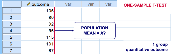
One-Sample T-Test Example

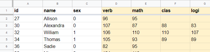
A school director thinks his students perform poorly due to low IQ scores. Now, most IQ tests have been calibrated to have a mean of 100 points in the general population. So the question is does the student population have a mean IQ score of 100? Now, our school has 1,114 students and the IQ tests are somewhat costly to administer. Our director therefore draws a simple random sample of N = 38 students and tests them on 4 IQ components:

• verb (Verbal Intelligence )
• math (Mathematical Ability )
• clas (Classification Skills )
• logi (Logical Reasoning Skills)

The raw data thus collected are in this Googlesheet, partly shown below. Note that a couple of scores are missing due to illness and unknown reasons.

Null Hypothesis

We'll try to demonstrate that our students have low IQ scores by rejecting the null hypothesis that the mean IQ score for the entire student population is 100 for each of the 4 IQ components measured. Our main challenge is that we only have data on a sample of 38 students from a population of N = 1,114. But let's first just look at some descriptive statistics for each component:

• N - sample size;
• M - sample mean and
• SD - sample standard deviation.

Descriptive Statistics

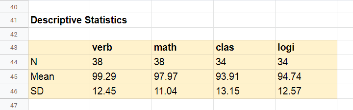
Our first basic conclusion is that our 38 students score lower than 100 points on all 4 IQ components. The differences for verb (99.29) and math (97.97) are small. Those for clas (93.91) and logi (94.74) seem somewhat more serious.
Now, our sample of 38 students may obviously come up with slightly different means than our population of N = 1,114. So what can we (not) conclude regarding our population? We'll try to generalize these sample results to our population with 2 different approaches:

• Statistical significance: how likely are these sample means if the population means are really all 100 points?
• Confidence intervals: given the sample results, what are likely ranges for the population means?

Both approaches require some assumptions so let's first look into those.

Assumptions

The assumptions required for our one-sample t-tests are

1. independent observations and
2. normality: the IQ scores must be normally distributed in the entire population.

Do our data meet these assumptions? First off,

1. our students didn't interact during their tests. Therefore, our observations are likely to be independent.
2. Normality is only needed for small sample sizes, say N < 25 or so. For the data at hand, normality is no issue. For smaller sample sizes, you could evaluate the normality assumption by

• inspecting if the histograms roughly follow normal curves,
• inspecting if both skewness and kurtosis are close to 0 and
• running a Shapiro-Wilk test or a Kolmogorov-Smirnov test.

However, the data at hand meet all assumptions so let's now look into the actual tests.

Formulas

If we'd draw many samples of students, such samples would come up with different means. We can compute the standard deviation of those means over hypothesized samples: the standard error of the mean or \(SE_{mean}\) $$SE_{mean} = \frac{SD}{\sqrt{N}}$$
for our first IQ component, this results in $$SE_{mean} = \frac{12.45}{\sqrt{38}} = 2.02$$
Our null hypothesis is that the population mean, \(\mu_0 = 100\). If this is true, then the average sample mean should also be 100. We now basically compute the z-score for our sample mean: the test statistic \(t\) $$t = \frac{M - \mu_0}{SE_{mean}}$$
for our first IQ component, this results in $$t = \frac{99.29 - 100}{2.02} = -0.35$$
If the assumptions are met, \(t\) follows a t distribution with the degrees of freedom or \(df\) given by $$df = N - 1$$
For a sample of 38 respondents, this results in $$df = 38 - 1 = 37$$
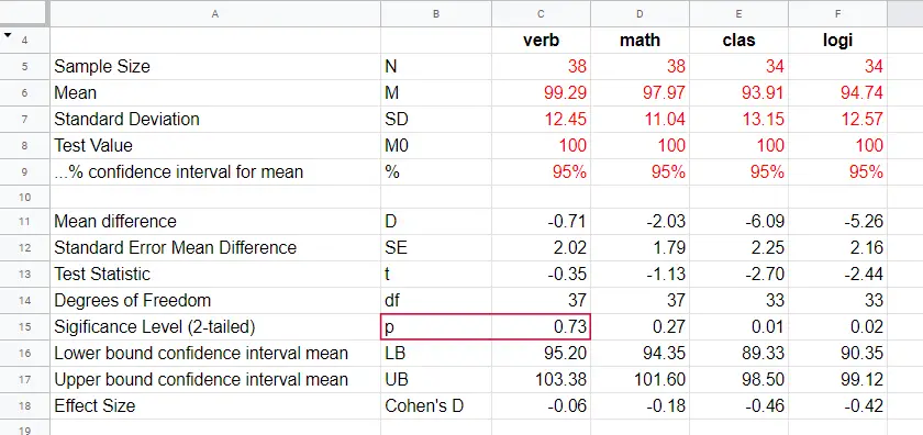
Given \(t\) and \(df\), we can simply look up that the 2-tailed significance level \(p\) = 0.73 in this Googlesheet, partly shown below.

Interpretation

As a rule of thumb, we reject the null hypothesis if p < 0.05. We just found that p = 0.73 so we don't reject our null hypothesis: given our sample data, the population mean being 100 is a credible statement.

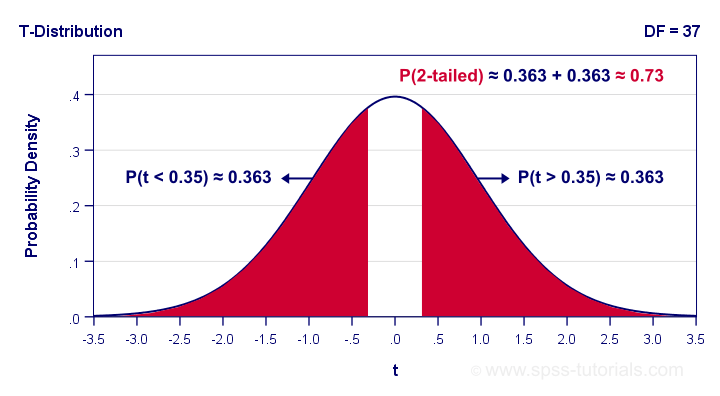
So precisely what does p = 0.73 mean? Well, it means there's a 0.73 (or 73%) probability that t < -0.35 or t > 0.35. The figure below illustrates how this probability results from the sampling distribution, t(37).

Next, remember that t is just a standardized mean difference. For our data, t = -0.35 corresponds to a difference of -0.71 IQ points. Therefore, p = 0.73 means that there's a 0.73 probability of finding an absolute mean difference of at least 0.71 points. Roughly speaking, the sample mean we found is likely to occur
if the null hypothesis is true.

Effect Size

The only effect size measure for a one-sample t-test is Cohen’s D defined as $$Cohen's\;D = \frac{M - \mu_0}{SD}$$

For our first IQ test component, this results in $$Cohen's\;D = \frac{99.29 - 100}{12.45} = -0.06$$

Some general conventions are that

• | Cohen’s D | = 0.20 indicates a small effect size;
• | Cohen’s D | = 0.50 indicates a medium effect size;
• | Cohen’s D | = 0.80 indicates a large effect size.

This means that Cohen’s D = -0.06 indicates a negligible effect size for our first test component. Cohen’s D is completely absent from SPSS except for SPSS 27. However, we can easily obtain it from JASP. The JASP output below shows the effect sizes for all 4 IQ test components.

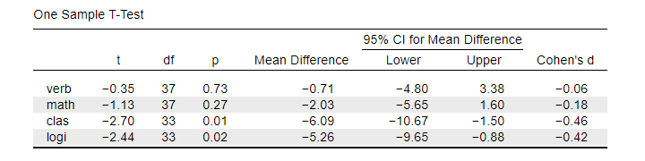
Note that the last 2 IQ components -clas and logi- almost have medium effect sizes. These are also the 2 components whose means differ significantly from 100: p < 0.05 for both means (third table column).

Confidence Intervals for Means

Our data came up with sample means for our 4 IQ test components. Now, we know that sample means typically differ somewhat from their population counterparts. So what are likely ranges for the population means we're after? This is often answered by computing 95% confidence intervals. We'll demonstrate the procedure for our last IQ component, logical reasoning.
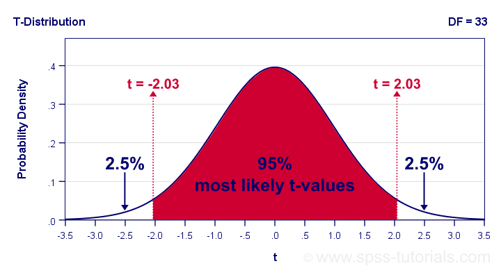
Since we've 34 observations, t follows a t-distribution with df = 33. We'll first look up which t-values enclose the most likely 95% from the inverse t-distribution. We'll do so by typing =T.INV(0.025,33) into any cell of a Googlesheet, which returns -2.03. Note that 0.025 is 2.5%. This is because the 5% most unlikely values are divided over both tails of the distribution as shown below.

Now, our t-value of -2.03 estimates that our 95% of our sample means fluctuate between ± 2.03 standard errors denoted by \(SE_{mean}\) For our last IQ component, $$SE_{mean} = \frac{12.57}{\sqrt34} = 2.16 $$

We now know that 95% of our sample means are estimated to fluctuate between ± 2.03 · 2.16 = 4.39 IQ test points. Last, we combine this fluctuation with our observed sample mean of 94.74: $$CI_{95\%} = [94.74 - 4.39,94.74 + 4.39] = [90.35,99.12]$$

Note that our 95% confidence interval does not enclose our hypothesized population mean of 100. This implies that we'll reject this null hypothesis at α = 0.05. We don't even need to run the actual t-test for drawing this conclusion.

APA Style Reporting

A single t-test is usually reported in text as in “The mean for verbal skills did not differ from 100,
t(37) = -0.35, p = 0.73, Cohen’s D = 0.06.” For multiple tests, a simple overview table as shown below is recommended. We feel that confidence intervals for means (not mean differences) should also be included. Since the APA does not mention these, we left them out for now.

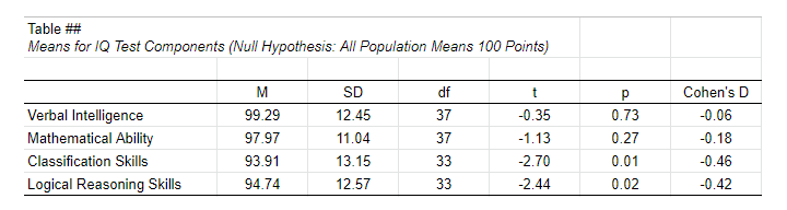APA Style Reporting Table Example for One-Sample T-Tests

Right. Well, I can't think of anything else that is relevant regarding the one-sample t-test. If you do, don't be shy. Just write us a comment below. We're always happy to hear from you!

Thanks for reading!