Most data analysts are familiar with post hoc tests for ANOVA. Oddly, post hoc tests for the chi-square independence test are not widely used. This tutorial walks you through 2 options for obtaining and interpreting them in SPSS.
- Option 1 - CROSSTABS
- CROSSTABS with Pairwise Z-Tests Output
- Option 2 - Custom Tables
- Custom Tables with Pairwise Z-Tests Output
- Can these Z-Tests be Replicated?
Example Data
A sample of N = 300 respondents were asked about their education level and marital status. The data thus obtained are in edu-marit.sav. All examples in this tutorial use this data file.
Chi-Square Independence Test
Right. So let's see if education level and marital status are associated in the first place: we'll run a chi-square independence test with the syntax below. This also creates a contingency table showing both frequencies and column percentages.
crosstabs marit by educ
/cells count column
/statistics chisq.
Let's first take a look at the actual test results shown below.
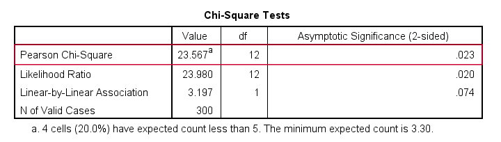
First off, we reject the null hypothesis of independence: education level and marital status are associated, χ2(12) = 23.57, p = 0.023. Note that that SPSS wrongfully reports this 1-tailed significance as a 2-tailed significance. But anyway, what we really want to know is precisely which percentages differ significantly from each other?
Option 1 - CROSSTABS
We'll answer this question by slightly modifying our syntax: adding BPROP (short for “Bonferroni proportions”) to the /CELLS subcommand does the trick.
crosstabs marit by educ
/cells count column bprop. /*bprop = Bonferroni adjusted z-tests for column proportions.
Running this simple syntax results in the table shown below.
CROSSTABS with Pairwise Z-Tests Output
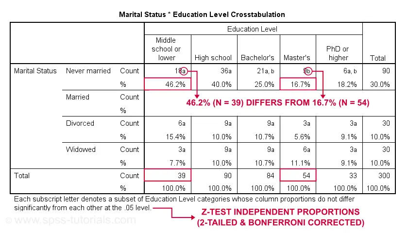
First off, take a close look at the table footnote: “Each subscript letter denotes a subset of Education Level categories whose column proportions do not differ significantly from each other at the .05 level.”
These conclusions are based on z-tests for independent proportions. These also apply to the percentages shown in the table: within each row, each possible pair of percentages is compared using a z-test. If they don't differ, they get a similar subscript. Reversely,
within each row, percentages that don't share a subscript
are significantly different.
For example, the percentage of people with middle school who never married is 46.2% and its frequency of n = 18 is labeled “a”. For those with a Master’s degree, 16.7% never married and its frequency of 9 is not labeled “a”. This means that 46.2% differs significantly from 16.7%.
The frequency of people with a Bachelor’s degree who never married (n = 21 or 25.0%) is labeled both “a” and “b”. It doesn't differ significantly from any cells labeled “a”, “b” or both. Which are all cells in this table row.
Now, a Bonferroni correction is applied for the number of tests within each row. This means that for \(k\) columns,
$$P_{bonf} = P\cdot\frac{k(k - 1)}{2}$$
where
- \(P_{bonf}\) denotes a Bonferroni corrected p-value and
- \(P\) denotes a “normal” (uncorrected) p-value.
Right, now our table has 5 education levels as columns so
$$P_{bonf} = P\cdot\frac{5(5 - 1)}{2} = P \cdot 10$$
which means that each p-value is multiplied by 10 and only then compared to alpha = 0.05. Or -reversely- only z-tests yielding an uncorrected p < 0.005 are labeled “significant”. This holds for all tests reported in this table. I'll verify these claims later on.
Option 2 - Custom Tables
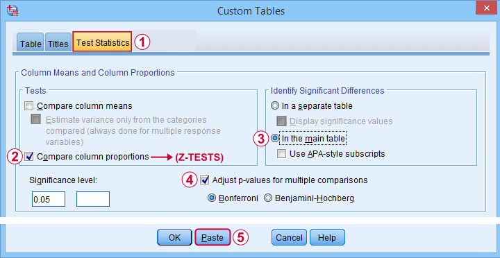
A second option for obtaining “post hoc tests” for chi-square tests are Custom Tables. They're found under
![]()
![]() but only if you have a Custom Tables license. The figure below suggests some basic steps.
but only if you have a Custom Tables license. The figure below suggests some basic steps.
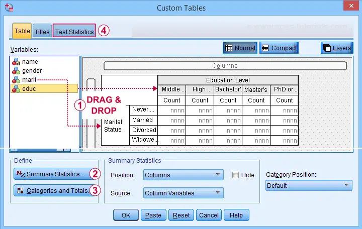
 You probably want to select both frequencies and column percentages for education level.
 We recommend you add totals for education levels as well.
Next, our z-tests are found in the Test Statistics tab shown below.
Completing these steps results in the syntax below.
CTABLES
/VLABELS VARIABLES=marit educ DISPLAY=DEFAULT
/TABLE marit BY educ [COUNT 'N' F40.0, COLPCT.COUNT '%' PCT40.1]
/CATEGORIES VARIABLES=marit ORDER=A KEY=VALUE EMPTY=INCLUDE TOTAL=YES POSITION=AFTER
/CATEGORIES VARIABLES=educ ORDER=A KEY=VALUE EMPTY=INCLUDE
/CRITERIA CILEVEL=95
/COMPARETEST TYPE=PROP ALPHA=0.05 ADJUST=BONFERRONI ORIGIN=COLUMN INCLUDEMRSETS=YES
CATEGORIES=ALLVISIBLE MERGE=YES STYLE=SIMPLE SHOWSIG=NO.
Custom Tables with Pairwise Z-Tests Output
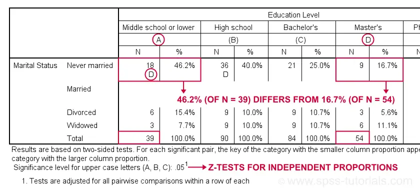
Let's first try and understand what the footnote says: “Results are based on two-sided tests. For each significant pair, the key of the category with the smaller column proportion appears in the category with the larger column proportion. Significance level for upper case letters (A, B, C): .05. Tests are adjusted for all pairwise comparisons within a row of each innermost subtable using the Bonferroni correction.”
Now, for normal 2-way contingency tables, the “innermost subtable” is simply the entire table. Within each row, each possible pair of column proportions is compared using a z-test. If 2 proportions differ significantly, then the higher is flagged with the column letter of the lower. Somewhat confusingly, SPSS flags the frequencies instead of the percentages.
In the first row (never married),
the D in column A indicates that these 2 percentages
differ significantly:
the percentage of people who never married is significantly higher for those who only completed middle school (46.2% from n = 39) than for those who completed a Master’s degree (16.7% from n = 54).
Again, all z-tests use α = 0.05 after Bonferroni correcting their p-values for the number of columns in the table. For our example table with 5 columns, each p-value is multiplied by \(0.5\cdot5(5 - 1) = 10\) before evaluating if it's smaller than the chosen alpha level of 0.05.
Can these Z-Tests be Replicated?
Yes. They can.
Custom Tables has an option to create a table containing the exact p-values for all pairwise z-tests. It's found in the Test Statistics tab. Selecting it results in the syntax below.
CTABLES
/VLABELS VARIABLES=marit educ DISPLAY=DEFAULT
/TABLE marit BY educ [COUNT 'N' F40.0, COLPCT.COUNT '%' PCT40.1]
/CATEGORIES VARIABLES=marit ORDER=A KEY=VALUE EMPTY=INCLUDE TOTAL=YES POSITION=AFTER
/CATEGORIES VARIABLES=educ ORDER=A KEY=VALUE EMPTY=INCLUDE
/CRITERIA CILEVEL=95
/COMPARETEST TYPE=PROP ALPHA=0.05 ADJUST=BONFERRONI ORIGIN=COLUMN INCLUDEMRSETS=YES
CATEGORIES=ALLVISIBLE MERGE=NO STYLE=SIMPLE SHOWSIG=YES.
Exact P-Values for Z-Tests
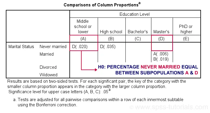
For the first row (never married), SPSS claims that the Bonferroni corrected p-value for comparing column percentages A and D is p = 0.020. For our example table, this implies an uncorrected p-value of p = 0.0020.
We replicated this result with an Excel z-test calculator. Taking the Bonferroni correction into account, it comes up with the exact same p-value as SPSS.
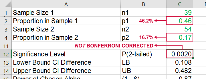
All other p-values reported by SPSS were also exactly replicated by our Excel calculator.
I hope this tutorial has been helpful for obtaining and understanding pairwise z-tests for contingency tables. If you've any questions or feedback, please throw us a comment below.
Thanks for reading!
THIS TUTORIAL HAS 35 COMMENTS:
By Ruben Geert van den Berg on March 26th, 2022
Hi Kael!
Please read the table footnotes very carefully:
Numbers sharing subscripts do not differ significantly.
So 18ab does not differ from 36ab, 9b or 6a - they all share at least one subscript.
However, 9b and 6a do differ as these don't share any subscripts.
Hope that helps!
Ruben
SPSS tutorials
By Jon Peck on April 19th, 2022
I disagree with your comment about Chi-squared being a one tail test. Even though it is only looking at one tail of the F distribution, it is considered to be a two-tail test, since it is just testing whether the frequencies differ.
CTABLES displays the significance results in the Count cells, because displaying the percentages is not required when doing the test.
Also, it's worth noting that CTABLES offers two choices for the multiple-testing correction. Bonferroni is the default, but it is very conservative. Especially if there are a lot of cells being compared, the Benjamini-Hochberg choice may be better in terms of the balance between Type 1 and Type 2 errors.
BF and BH are the most popular multiple hypothesis corrections, but there are others. The STATS PADJUST extension command, which is available from the Extension Hub, offers six methods. It also has the advantage that it can be used with the output from procedures that do not have multiple-testing corrections built in.
One other note: with CTABLES, if you want to highlight cells where there are significant differences, the SPSSINC MODIFY TABLES extension command can do this.
By Ruben Geert van den Berg on April 20th, 2022
Hi Jon!
To me, "p(2-tailed)" suggests that you could also choose to report 0.5 * p as "p(1-tailed)".
IMHO, we should simply report "p" whenever only one of these options can be taken seriously. If both are serious candidates, then "p(1/2-tailed)" is obviously the more explicit and -thus- better option.
If I follow your line of reasoning, then why doesn't SPSS report "Sig. (2-tailed)" for ANOVA results as well?
By the way, I think reporting "Sig." instead of "p" is not optimal anyway.
I've no outspoken opinion of which correction is "best". Do you have any solid reference on your claim that BH may be better than BF? If so, I'll happily advocate BH rather than BF.
In any case, I feel that most social scientists are overly obsessed with "significance". Perhaps that's because "significance" also has a normal language meaning which may be very different from "statistical significance".
IMHO, reporting CI's for effect sizes is a much more fruitful approach. Great to see that these were added to some extent to SPSS 27.
It's a real bummer, however, that many tests don't have any effect size measure in the first place, especially normality tests and distribution free ("nonparametric") tests.
By jon on April 20th, 2022
BF and BH control different things. If there are a lot of tests, it is hard for BF to show significance. Quoting from Wikipedia,
"The FDR [false discovery rate] concept was formally described by Yoav Benjamini and Yosef Hochberg in 1995[1] (BH procedure) as a less conservative and arguably more appropriate approach for identifying the important few from the trivial many effects tested. The FDR has been particularly influential, as it was the first alternative to the FWER [familywise error rate] to gain broad acceptance in many scientific fields"
" the false discovery rate (FDR) is a method of conceptualizing the rate of type I errors in null hypothesis testing when conducting multiple comparisons. FDR-controlling procedures are designed to control the FDR, which is the expected proportion of "discoveries" (rejected null hypotheses) that are false (incorrect rejections of the null)"
And from this site, https://www.biostathandbook.com/multiplecomparisons.html,
https://www.biostathandbook.com/multiplecomparisons.html
"The Bonferroni correction is appropriate when a single false positive in a set of tests would be a problem. It is mainly useful when there are a fairly small number of multiple comparisons and you're looking for one or two that might be significant. However, if you have a large number of multiple comparisons and you're looking for many that might be significant, the Bonferroni correction may lead to a very high rate of false negatives. "
If there are only a few tests, the difference is [sic] insignificant, but since BF requires dividing the p value by the number of tests, it quickly becomes very hard to show significance. The often cited usage where there are literally thousands of tests is unlikely to occur in social science contexts, but even with just a handful of tests, the balance between Type 1 and Type 2 error becomes pretty important IMO.
By Leta on April 24th, 2023
great it's very important for all