Categorical variables can't readily be used as predictors in multiple regression analysis. They must be split up into dichotomous variables known as “dummy variables”. This tutorial offers a simple tool for creating them.
- Example Data File
- Prerequisites and Installation
- Example I - Numeric Categorical Variable
- Example II - Categorical String Variable
Example Data File
We'll demonstrate our tool on 2 examples: a numeric and a string variable. Both variables are in staff.sav, partly shown below.
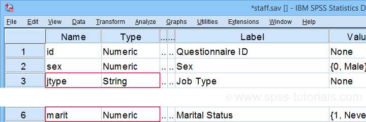
We encourage you to download and open this data file in SPSS and replicate the examples we'll present.
Prerequisites and Installation
Our tool requires SPSS version 24 or higher. Also, the SPSS Python 3 essentials must be installed (usually the case with recent SPSS versions).
Next, click SPSS_TUTORIALS_DUMMIFY.spe in order to download our tool. For installing it, navigate to
![]() as shown below.
as shown below.
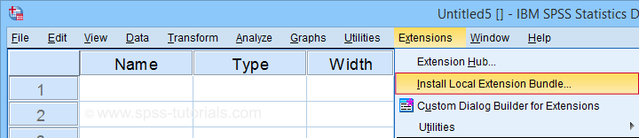
In the dialog that opens, navigate to the downloaded .spe file and install it. SPSS will then confirm that the extension was successfully installed under
![]()
Example I - Numeric Categorical Variable
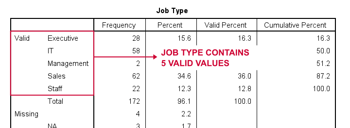
Let's now dummify Marital Status. Before doing so, we recommend you first inspect its basic frequency distribution as shown below.
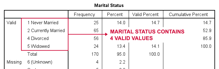
Importantly, note that Marital Status contains 4 valid (non missing) values. As we'll explain later on, we always need to exclude one category, known as the reference category. We'll therefore create 3 dummy variables to represent our 4 categories.
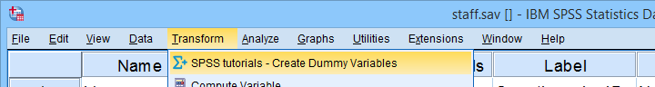
We'll do so by navigating to
![]() as shown below.
as shown below.
Let's now fill out the dialog that pops up.
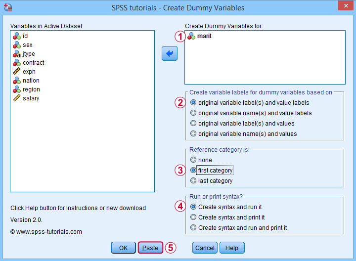
 We choose the first category (“Never Married”) as our reference category. Completing these results in the syntax below. Let's run it.
SPSS TUTORIALS DUMMIFY VARIABLES=marit
/OPTIONS NEWLABELS=LABLAB REFCAT=FIRST ACTION=RUN.
Result
Our tool has now created 3 dummy variables in the active dataset. Let's compare them to the value labels of our original variable, Marital Status.
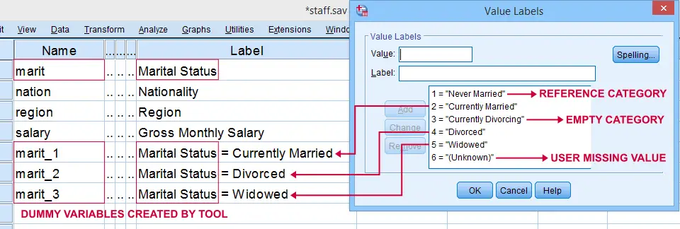
First note that the variable names for our dummy variables are the original variable name plus an integer suffix. These suffixes don't usually correspond to the categories they represent.
Instead, these categories are found in the variable labels for our dummy variables. In this example, they are based on the variable and value labels in Marital Status.
Next, note that some categories were skipped for the following reasons:
- no dummy variable was created for “Never Married” because we chose it as our reference category;
- no dummy variable was created for “Currently Divorcing” because it doesn't actually occur in our dataset;
- no dummy variable was created for “(Unknown)” because it is a user missing value.
Now the big question is:
are these results correct?
An easy way to confirm that they are indeed correct is actually running a dummy variable regression. We'll then run the exact same analysis with a basic ANOVA.
For example, let's try and predict Salary from Marital Status via both methods by running the syntax below.
regression
/dependent salary
/method enter marit_1 to marit_3.
*Compare mean salaries by marital status via ANOVA.
means salary by marit
/statistics anova.
First note that the regression r-square of 0.089 is identical to the eta squared of 0.089 in our ANOVA results. This makes sense because they both indicate the proportion of variance in Salary accounted for by Marital Status.
Also, our ANOVA comes up with a significance level of p = 0.002 just as our regression analysis does. We could even replicate the regression B-coefficients and their confidence intervals via ANOVA (we'll do so in a later tutorial). But for now, let's just conclude that the results are correct.
Example II - Categorical String Variable
Let's now dummify Job Type, a string variable. Again, we'll start off by inspecting its frequencies and we'll probably want to specify some missing values. As discussed in SPSS - Missing Values for String Variables, doing so is cumbersome but the syntax below does the job.
frequencies jtype.
*Change '(Unknown)' into 'NA'.
recode jtype ( '(Unknown)' = 'NA').
*Set empty string value and 'NA' as user missing values.
missing values jtype ('','NA').
*Reinspect basic frequency table.
frequencies jtype.
Result
Again, we'll first navigate to
![]() and we'll fill in the dialog as shown below.
and we'll fill in the dialog as shown below.
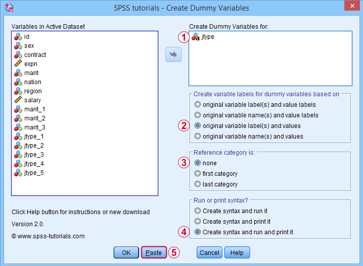
 For string variables, the values themselves usually describe their categories. We therefore throw values (instead of value labels) into the variable labels for our dummy variables.
If we neither want the first nor the last category as reference, we'll select “none”. In this case, we must manually exclude one of these dummy variables from the regression analysis that follows.
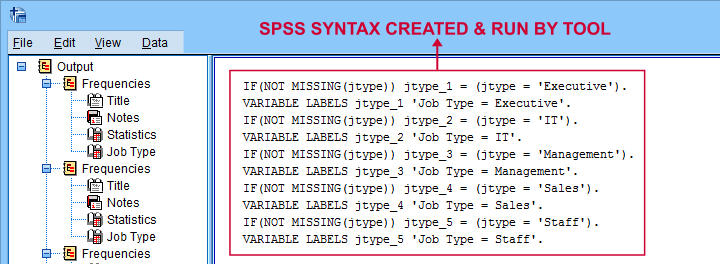
 Besides creating dummy variables, we may also want to inspect the syntax that's created and run by the tool. We may also copy, paste, edit and run it from a syntax window instead of having our tool do that for us.
Completing these steps result in the syntax below.
SPSS TUTORIALS DUMMIFY VARIABLES=jtype
/OPTIONS NEWLABELS=LABVAL REFCAT=NONE ACTION=BOTH.
Result
Besides creating 5 dummy variables, our tool also prints the syntax that was used in the output window as shown below.
Finally, if you didn't choose any reference category, you must exclude one of the dummy variables from your regression analysis. The syntax below shows what happens if you don't.
regression
/dependent salary
/method enter jtype_1 jtype_2 jtype_3 jtype_4 jtype_5.
*Compare salaries by Job Type right way: reference category = 4 (sales).
regression
/dependent salary
/method enter jtype_1 jtype_2 jtype_3 jtype_5.
The first example is a textbook illustration of perfect multicollinearity: the score on some predictor can be perfectly predicted from some other predictor(s). This makes sense: a respondent scoring 0 on the first 4 dummies must score 1 on the last (and reversely).
In this situation, B-coefficients can't be estimated. Therefore, SPSS excludes a predictor from the analysis as shown below.
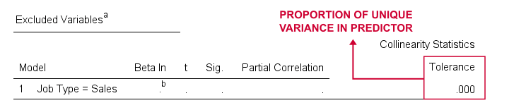
Note that tolerance is the proportion of variance in a predictor that can not be accounted for by other predictors in the model. A tolerance of 0.000 thus means that some predictor can be 100% -or perfectly- predicted from the other predictors.
Thanks for reading!
THIS TUTORIAL HAS 21 COMMENTS:
By christopher Anyuzu on August 5th, 2021
I would learn more about spss
By bobby cunningham on April 8th, 2022
Great tutorial to help to understand my data analysis better.
By Ola Johansson on April 25th, 2022
Hi, I have used your Dummy tool successfully on SPSS version 27, but cannot get it to work with version 28. Is this a common problem? Anyone know how to resolve it?
By Ruben Geert van den Berg on April 25th, 2022
No, I've been using the tool on SPSS 25 and 28 without any issues.
Could you give me some more details? Exactly what warnings/errors are you seeing?
By Guankeyi Chuchu Guanbei on July 2nd, 2024
I'm interested in learning IBM SPSS for accurate data analysis. If I can be connected to someone for guidance