- What is Factor Analysis?
- Quick Data Checks
- Running Factor Analysis in SPSS
- SPSS Factor Analysis Output
- Adding Factor Scores to Our Data
What is Factor Analysis?
Factor analysis examines which underlying factors are measured
by a (large) number of observed variables.
Such “underlying factors” are often variables that are difficult to measure such as IQ, depression or extraversion. For measuring these, we often try to write multiple questions that -at least partially- reflect such factors. The basic idea is illustrated below.
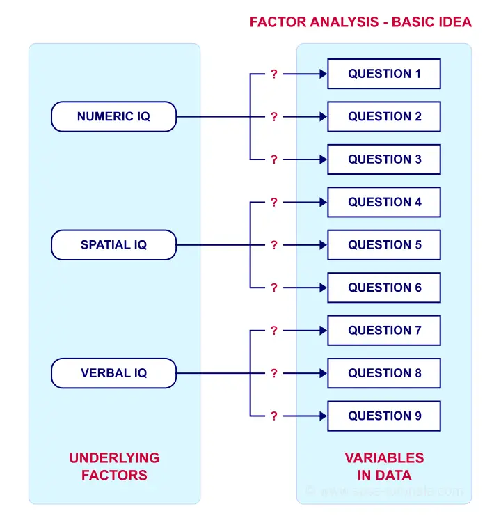
Now, if questions 1, 2 and 3 all measure numeric IQ, then the Pearson correlations among these items should be substantial: respondents with high numeric IQ will typically score high on all 3 questions and reversely.
The same reasoning goes for questions 4, 5 and 6: if they really measure “the same thing” they'll probably correlate highly.
However, questions 1 and 4 -measuring possibly unrelated traits- will not necessarily correlate. So if my factor model is correct, I could expect the correlations to follow a pattern as shown below.
Confirmatory Factor Analysis
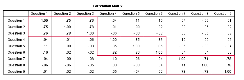
Right, so after measuring questions 1 through 9 on a simple random sample of respondents, I computed this correlation matrix. Now I could ask my software if these correlations are likely, given my theoretical factor model. In this case, I'm trying to confirm a model by fitting it to my data. This is known as “confirmatory factor analysis”.
SPSS does not include confirmatory factor analysis but those who are interested could take a look at AMOS.
Exploratory Factor Analysis
But what if I don't have a clue which -or even how many- factors are represented by my data? Well, in this case, I'll ask my software to suggest some model given my correlation matrix. That is, I'll explore the data (hence, “exploratory factor analysis”). The simplest possible explanation of how it works is that
the software tries to find groups of variables
that are highly intercorrelated.
Each such group probably represents an underlying common factor. There's different mathematical approaches to accomplishing this but the most common one is principal components analysis or PCA. We'll walk you through with an example.
Research Questions and Data
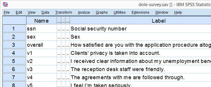
A survey was held among 388 applicants for unemployment benefits. The data thus collected are in dole-survey.sav, part of which is shown below.
The survey included 16 questions on client satisfaction. We think these measure a smaller number of underlying satisfaction factors but we've no clue about a model. So our research questions for this analysis are:
- how many factors are measured by our 16 questions?
- which questions measure similar factors?
- which satisfaction aspects are represented by which factors?
Quick Data Checks
Now let's first make sure we have an idea of what our data basically look like. We'll inspect the frequency distributions with corresponding bar charts for our 16 variables by running the syntax below.
set
tnumbers both /* show values and value labels in output tables */
tvars both /* show variable names but not labels in output tables */
ovars names. /* show variable names but not labels in output outline */
*Basic frequency tables with bar charts.
frequencies v1 to v20
/barchart.
Result
This very minimal data check gives us quite some important insights into our data:
- All frequency distributions look plausible. We don't see anything weird in our data.
- All variables are
 positively coded: higher values always indicate more positive sentiments.
 - All variables have
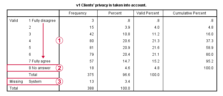
 a value 8 (“No answer”) which we need to set as a user missing value.
 - All variables have some
 system missing values too but the extent of missingness isn't too bad.
A somewhat annoying flaw here is that we don't see variable names for our bar charts in the output outline.
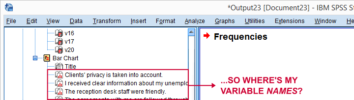
If we see something unusual in a chart, we don't easily see which variable to address. But in this example -fortunately- our charts all look fine.
So let's now set our missing values and run some quick descriptive statistics with the syntax below.
missing values v1 to v20 (8).
*Inspect valid N for each variable.
descriptives v1 to v20.
Result
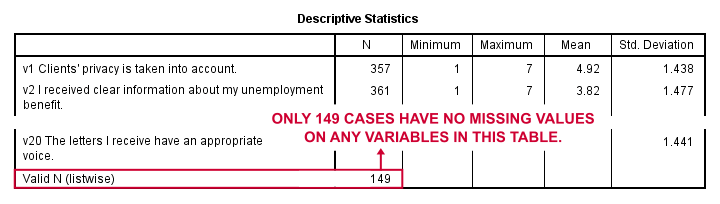
Note that none of our variables have many -more than some 10%- missing values. However, only 149 of our 388 respondents have zero missing values on the entire set of variables. This is very important to be aware of as we'll see in a minute.
Running Factor Analysis in SPSS
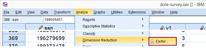
Let's now navigate to
![]()
![]() as shown below.
as shown below.
In the dialog that opens, we have a ton of options. For a “standard analysis”, we'll select the ones shown below. If you don't want to go through all dialogs, you can also replicate our analysis from the syntax below.
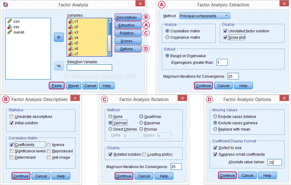
 Avoid “Exclude cases listwise” here as it'll only include our 149 “complete” respondents in our factor analysis. Clicking results in the syntax below.
SPSS Factor Analysis Syntax
set tvars both.
*Initial factor analysis as pasted from menu.
FACTOR
/VARIABLES v1 v2 v3 v4 v5 v6 v7 v8 v9 v11 v12 v13 v14 v16 v17 v20
/MISSING PAIRWISE /*IMPORTANT!*/
/PRINT INITIAL CORRELATION EXTRACTION ROTATION
/FORMAT SORT BLANK(.30)
/PLOT EIGEN
/CRITERIA MINEIGEN(1) ITERATE(25)
/EXTRACTION PC
/CRITERIA ITERATE(25)
/ROTATION VARIMAX
/METHOD=CORRELATION.
Factor Analysis Output I - Total Variance Explained
Right. Now, with 16 input variables, PCA initially extracts 16 factors (or “components”). Each component has a quality score called an Eigenvalue. Only components with high Eigenvalues are likely to represent real underlying factors.
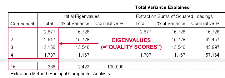
So what's a high Eigenvalue? A common rule of thumb is to select components whose Eigenvalues are at least 1. Applying this simple rule to the previous table answers our first research question: our 16 variables seem to measure 4 underlying factors.
This is because only our first 4 components have Eigenvalues of at least 1. The other components -having low quality scores- are not assumed to represent real traits underlying our 16 questions. Such components are considered “scree” as shown by the line chart below.
Factor Analysis Output II - Scree Plot
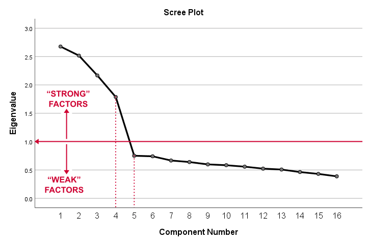
A scree plot visualizes the Eigenvalues (quality scores) we just saw. Again, we see that the first 4 components have Eigenvalues over 1. We consider these “strong factors”. After that -component 5 and onwards- the Eigenvalues drop off dramatically. The sharp drop between components 1-4 and components 5-16 strongly suggests that 4 factors underlie our questions.
Factor Analysis Output III - Communalities
So to what extent do our 4 underlying factors account for the variance of our 16 input variables? This is answered by the r square values which -for some really dumb reason- are called communalities in factor analysis.
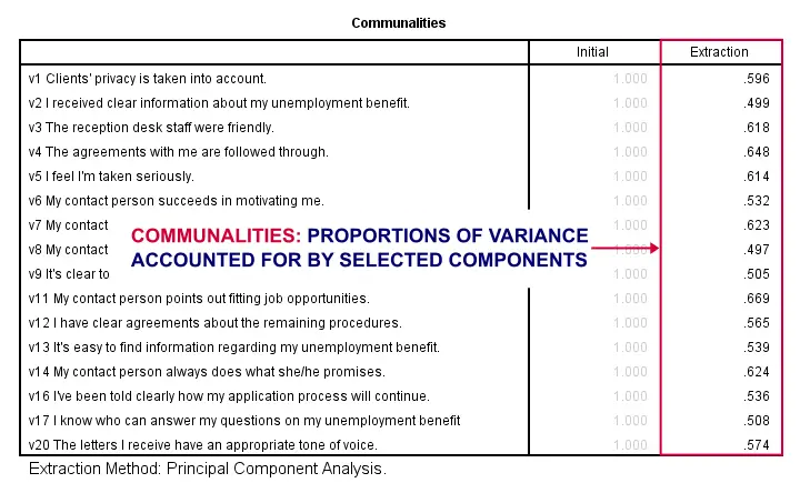
Right. So if we predict v1 from our 4 components by multiple regression, we'll find r square = 0.596 -which is v1’ s communality. Variables having low communalities -say lower than 0.40- don't contribute much to measuring the underlying factors.
You could consider removing such variables from the analysis. But keep in mind that doing so changes all results. So you'll need to rerun the entire analysis with one variable omitted. And then perhaps rerun it again with another variable left out.
If the scree plot justifies it, you could also consider selecting an additional component. But don't do this if it renders the (rotated) factor loading matrix less interpretable.
Factor Analysis Output IV - Component Matrix
Thus far, we concluded that our 16 variables probably measure 4 underlying factors. But which items measure which factors? The component matrix shows the Pearson correlations between the items and the components. For some dumb reason, these correlations are called factor loadings.
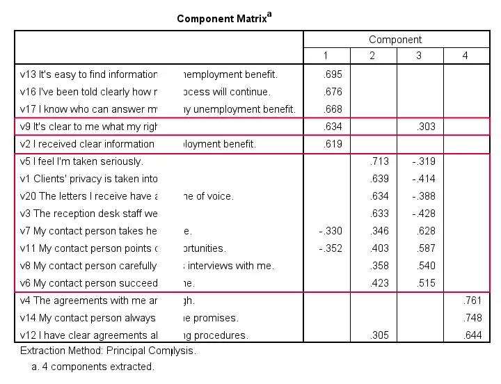
Ideally, we want each input variable to measure precisely one factor. Unfortunately, that's not the case here. For instance, v9 measures (correlates with) components 1 and 3. Worse even, v3 and v11 even measure components 1, 2 and 3 simultaneously. If a variable has more than 1 substantial factor loading, we call those cross loadings. And we don't like those. They complicate the interpretation of our factors.
The solution for this is rotation: we'll redistribute the factor loadings over the factors according to some mathematical rules that we'll leave to SPSS. This redefines what our factors represent. But that's ok. We hadn't looked into that yet anyway.
Now, there's different rotation methods but the most common one is the varimax rotation, short for “variable maximization. It tries to redistribute the factor loadings such that each variable measures precisely one factor -which is the ideal scenario for understanding our factors. And as we're about to see, our varimax rotation works perfectly for our data.
Factor Analysis Output V - Rotated Component Matrix
Our rotated component matrix (below) answers our second research question: “which variables measure which factors?”
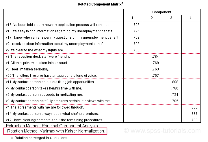
Our last research question is: “what do our factors represent?” Technically, a factor (or component) represents whatever its variables have in common. Our rotated component matrix (above) shows that our first component is measured by
- v17 - I know who can answer my questions on my unemployment benefit.
- v16 - I've been told clearly how my application process will continue.
- v13 - It's easy to find information regarding my unemployment benefit.
- v2 - I received clear information about my unemployment benefit.
- v9 - It's clear to me what my rights are.
Note that these variables all relate to the respondent receiving clear information. Therefore, we interpret component 1 as “clarity of information”. This is the underlying trait measured by v17, v16, v13, v2 and v9.
After interpreting all components in a similar fashion, we arrived at the following descriptions:
- Component 1 - “Clarity of information”
- Component 2 - “Decency and appropriateness”
- Component 3 - “Helpfulness contact person”
- Component 4 - “Reliability of agreements”
We'll set these as variable labels after actually adding the factor scores to our data.
Adding Factor Scores to Our Data
It's pretty common to add the actual factor scores to your data. They are often used as predictors in regression analysis or drivers in cluster analysis. SPSS FACTOR can add factor scores to your data but this is often a bad idea for 2 reasons:
- factor scores will only be added for cases without missing values on any of the input variables. We saw that this holds for only 149 of our 388 cases;
- factor scores are z-scores: their mean is 0 and their standard deviation is 1. This complicates their interpretation.
In many cases, a better idea is to compute factor scores as means over variables measuring similar factors. Such means tend to correlate almost perfectly with “real” factor scores but they don't suffer from the aforementioned problems. Note that you should only compute means over variables that have identical measurement scales.
It's also a good idea to inspect Cronbach’s alpha for each set of variables over which you'll compute a mean or a sum score. For our example, that would be 4 Cronbach's alphas for 4 factor scores but we'll skip that for now.
Computing and Labeling Factor Scores Syntax
compute fac_1 = mean(v16,v13,v17,v2,v9).
compute fac_2 = mean(v3,v1,v5,v20).
compute fac_3 = mean(v11,v7,v6,v8).
compute fac_4 = mean(v4,v14,v12).
*Label factors.
variable labels
fac_1 'Clarity of information'
fac_2 'Decency and appropriateness'
fac_3 'Helpfulness contact person'
fac_4 'Reliability of agreements'.
*Quick check.
descriptives fac_1 to fac_4.
Result
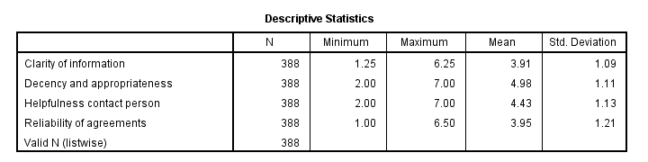
This descriptives table shows how we interpreted our factors. Because we computed them as means, they have the same 1 - 7 scales as our input variables. This allows us to conclude that
- “Decency and appropriateness” is rated best (roughly 5.0 out of 7 points) and
- “Clarity of information” is rated worst (roughly 3.9 out of 7 points).
Thanks for reading!
THIS TUTORIAL HAS 131 COMMENTS:
By Ruben Geert van den Berg on April 26th, 2022
Hi Jon, thanks for your feedback!
"The variable name information is available in the Chart Editor for the Frequencies bar charts, and they are in the same order as the preceding frequency tables."
Yes, but we typically use FA for a substantial number of items and in many cases, variable labels may be somewhat lengthy and have the same start ("Please indicate..."). So I still find it annoying that OVARS is somehow ignored here. Perhaps a better option is using /ORDER VARIABLE on the FREQUENCIES subcommand so the preceding freq tables indicate precisely which barchart we're seeing...
"FA is only appropriate for continuous (including dichotomous) variables."
Why does everybody mix up "continuous" with "quantitative"? A variable is continuous if and only if between each pair of values a third value exists. If that's not the case, it's discrete but it can still be quantitative.
An example are financial transactions: there doesn't exist any transaction between $0.01 and $0.02 so this variable is discrete, not continuous. However, it's perfectly quantitative and thus suitable for correlations/regression/whatever.
I think it's a bad habit to be sloppy regarding such terminology -even if text books and articles also mess things up (except for mathematical statistics which is perfectly clear and simple about such issues).
By Jon K Peck on April 26th, 2022
It's an interesting question what measurement level variables should have in factor analysis. Since FA doesn't actually involve statistical inference but rather just some linear algebra, this isn't obvious. However, since the model assumes the variables live in a Euclidean vector space and projects accordingly, the most plausible assumption is that the variables should be continuous - yes, continuous, not just quantitative.
By Ruben Geert van den Berg on April 27th, 2022
Interesting point.
However -and please do correct me if I'm wrong here- I believe a mere correlation matrix suffices -practically as well as theoretically- for running a (minimal) PCA.
I think Euclidean distances are only meaningful if they're based on 2+ variables having the same literal scales (kilos/dollars/seconds), right?
But what if I asked people
-how many books do you own?
-how many CDs do you own?
-how many DVDs do you own?
-how many ...
These are all quantitative (but undisputably discrete) variables and I think correlations -but not Euclidean distances- make perfect sense for them.
Would you argue that FA would be invalid on such a set of variables?
By Jon K Peck on April 27th, 2022
Well, in your example, some items will have higher variance than others, so standardizing the data might be called for. Of course, if analyzing the correlation matrix, this is already being done. As for discrete data, I doubt that anyone would FA nominal data, but the graininess of other data types would seem to me to matter if it is large relative to the dispersion of the variables, but as an algebraic rather than statistical technique, I don't know of a rule that one should apply. You might see the opposite situation with, say, crosstabs. You could tabulate continuous variables, but you probably wouldn't.
By Ruben Geert van den Berg on April 28th, 2022
Well, in your example, some items will have higher variance than others, so standardizing the data might be called for.
Of course, if analyzing the correlation matrix, this is already being done. As for discrete data, I doubt that anyone would FA nominal data, but the graininess of other data types would seem to me to matter if it is large relative to the dispersion of the variables, but as an algebraic rather than statistical technique, I don't know of a rule that one should apply.
You might see the opposite situation with, say, crosstabs. You could tabulate continuous variables, but you probably wouldn't.