- Method I - Histograms
- Excluding Outliers from Data
- Method II - Boxplots
- Method III - Z-Scores (with Reporting)
- Method III - Z-Scores (without Reporting)
Summary
Outliers are basically values that fall outside of a normal range for some variable. But what's a “normal range”? This is subjective and may depend on substantive knowledge and prior research. Alternatively, there's some rules of thumb as well. These are less subjective but don't always result in better decisions as we're about to see.
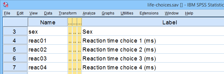
In any case: we usually want to exclude outliers from data analysis. So how to do so in SPSS? We'll walk you through 3 methods, using life-choices.sav, partly shown below.
 In this tutorial, we'll find outliers for these reaction time variables.
During this tutorial, we'll focus exclusively on reac01 to reac05, the reaction times in milliseconds for 5 choice trials offered to the respondents.
Method I - Histograms
Let's first try to identify outliers by running some quick histograms over our 5 reaction time variables. Doing so from SPSS’ menu is discussed in Creating Histograms in SPSS. A faster option, though, is running the syntax below.
frequencies reac01 to reac05
/histogram.
Result
Let's take a good look at the first of our 5 histograms shown below.
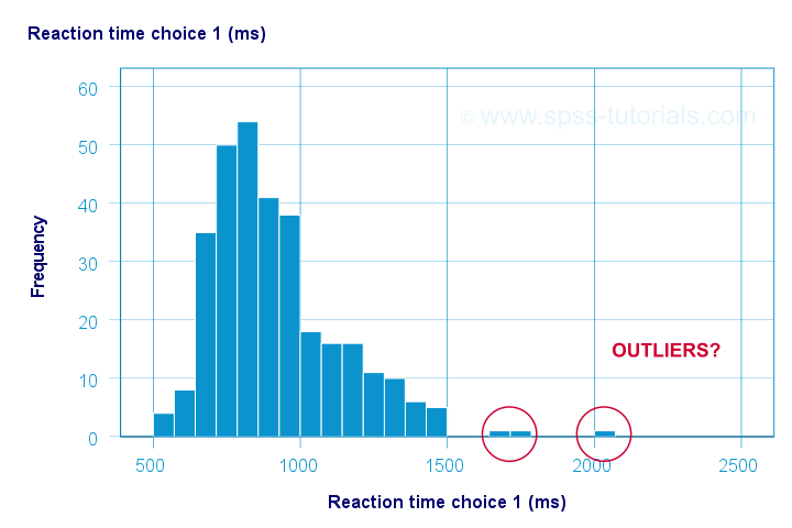
The “normal range” for this variable seems to run from 500 through 1500 ms. It seems that 3 scores lie outside this range. So are these outliers? Honestly, different analysts will make different decisions here. Personally, I'd settle for only excluding the score ≥ 2000 ms. So what's the right way to do so? And what about the other variables?
Excluding Outliers from Data
The right way to exclude outliers from data analysis is to specify them as user missing values. So for reaction time 1 (reac01), running missing values reac01 (2000 thru hi). excludes reaction times of 2000 ms and higher from all data analyses and editing. So what about the other 4 variables?
The histograms for reac02 and reac03 don't show any outliers.
For reac04, we see some low outliers as well as a high outlier. We can find which values these are in the bottom and top of its frequency distribution as shown below.
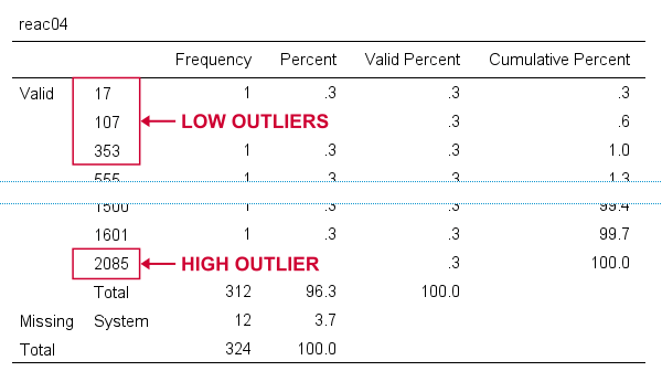 If we see any outliers in a histogram, we may look up the exact values in the corresponding frequency table.
We can exclude all of these outliers in one go by running missing values reac04 (lo thru 400,2085). By the way: “lo thru 400” means the lowest value in this variable (its minimum) through 400 ms.
For reac05, we see several low and high outliers. The obvious thing to do seems to run something like missing values reac05 (lo thru 400,2000 thru hi). But sadly, this only triggers the following error:
>There are too many values specified.
>The limit is three individual values or
>one value and one range of values.
>Execution of this command stops.
The problem here is that
you can't specify a low and a high
range of missing values in SPSS.
Since this is what you typically need to do, this is one of the biggest stupidities still found in SPSS today. A workaround for this problem is to
- RECODE the entire low range into some huge value such as 999999999;
- add the original values to a value label for this value;
- specify only a high range of missing values that includes 999999999.
The syntax below does just that and reruns our histograms to check if all outliers have indeed been correctly excluded.
recode reac05 (lo thru 400 = 999999999).
*Add value label to 999999999.
add value labels reac05 999999999 '(Recoded from 95 / 113 / 397 ms)'.
*Set range of high missing values.
missing values reac05 (2000 thru hi).
*Rerun frequency tables after excluding outliers.
frequencies reac01 to reac05
/histogram.
Result
First off, note that none of our 5 histograms show any outliers anymore; they're now excluded from all data analysis and editing. Also note the bottom of the frequency table for reac05 shown below.
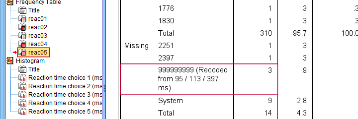 Low outliers after recoding and labelling are listed under Missing.
Even though we had to recode some values, we can still report precisely which outliers we excluded for this variable due to our value label.
Before proceeding to boxplots, I'd like to mention 2 worst practices for excluding outliers:
- removing outliers by changing them into system missing values. After doing so, we no longer know which outliers we excluded. Also, we're clueless why values are system missing as they don't have any value labels.
- removing entire cases -often respondents- because they have 1(+) outliers. Such cases typically have mostly “normal” data values that we can use just fine for analyzing other (sets of) variables.
Sadly, supervisors sometimes force their students to take this road anyway. If so, SELECT IF permanently removes entire cases from your data.
Method II - Boxplots
If you ran the previous examples, you need to close and reopen life-choices.sav before proceeding with our second method.
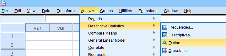
We'll create a boxplot as discussed in Creating Boxplots in SPSS - Quick Guide: we first navigate to
![]()
![]() as shown below.
as shown below.
Next, we'll fill in the dialogs as shown below.
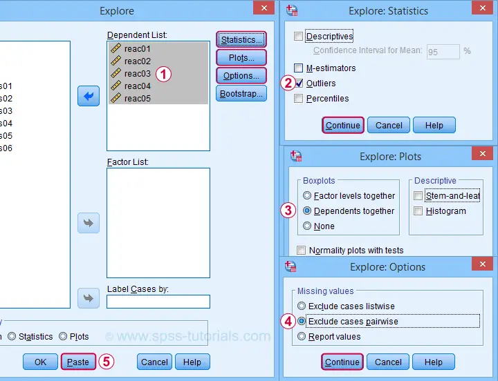
Completing these steps results in the syntax below. Let's run it.
EXAMINE VARIABLES=reac01 reac02 reac03 reac04 reac05
/PLOT BOXPLOT
/COMPARE VARIABLES
/STATISTICS EXTREME
/MISSING PAIRWISE
/NOTOTAL.
Result
Quick note: if you're not sure about interpreting boxplots, read up on Boxplots - Beginners Tutorial first.
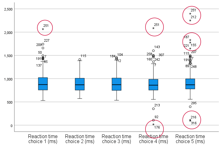
Our boxplot indicates some potential outliers for all 5 variables. But let's just ignore these and exclude only the extreme values that are observed for reac01, reac04 and reac05.
So, precisely which values should we exclude? We find them in the Extreme Values table. I like to copy-paste this into Excel. Now we can easily boldface all values that are extreme values according to our boxplot.
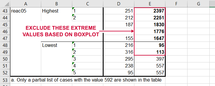 Copy-pasting the Extreme Values table into Excel allows you to easily boldface the exact outliers that we'll exclude.
Finally, we set these extreme values as user missing values with the syntax below. For a step-by-step explanation of this routine, look up Excluding Outliers from Data.
recode reac05 (lo thru 113 = 999999999).
*Label new value with original values.
add value labels reac05 999999999 '(Recoded from 95 / 113 ms)'.
*Set (ranges of) missing values for reac01, reac04 and reac05.
missing values
reac01 (2065)
reac04 (17,2085)
reac05 (1647 thru hi).
*Rerun boxplot and check if all extreme values are gone.
EXAMINE VARIABLES=reac01 reac02 reac03 reac04 reac05
/PLOT BOXPLOT
/COMPARE VARIABLES
/STATISTICS EXTREME
/MISSING PAIRWISE
/NOTOTAL.
Method III - Z-Scores (with Reporting)
A common approach to excluding outliers is to look up which values correspond to high z-scores. Again, there's different rules of thumb which z-scores should be considered outliers. Today, we settle for |z| ≥ 3.29 indicates an outlier. The basic idea here is that if a variable is perfectly normally distributed, then only 0.1% of its values will fall outside this range.
So what's the best way to do this in SPSS? Well, the first 2 steps are super simple:
- we add z-scores for all relevant variables to our data and
- see if their minima or maxima meet |z| ≥ 3.29.
Funnily, both steps are best done with a simple DESCRIPTIVES command as shown below.
descriptives reac01 to reac05
/save.
*Check min and max for z-scores.
descriptives zreac01 to zreac05.
Result
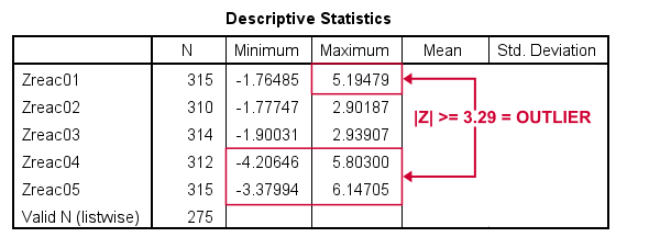 Minima and maxima for our newly computed z-scores.
Basic conclusions from this table are that
- reac01 has at least 1 high outlier;
- reac02 and reac03 don't have any outliers;
- reac04 and reac05 both have at least 1 low and 1 high outlier.
But which original values correspond to these high absolute z-scores? For each variable, we can run 2 simple steps:
- FILTER away cases having |z| < 3.29 (all non outliers);
- run a frequency table -now containing only outliers- on the original variable.
The syntax below does just that but uses TEMPORARY and SELECT IF for filtering out non outliers.
temporary.
select if(abs(zreac01) >= 3.29).
frequencies reac01.
temporary.
select if(abs(zreac04) >= 3.29).
frequencies reac04.
temporary.
select if(abs(zreac05) >= 3.29).
frequencies reac05.
*Save output because tables needed for reporting which outliers are excluded.
output save outfile = 'outlier-tables-01.spv'.
Result
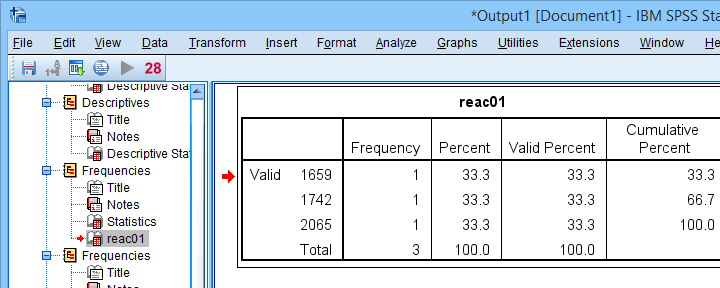 Finding outliers by filtering out all non outliers based on their z-scores.
Note that each frequency table only contains a handful of outliers for which |z| ≥ 3.29. We'll now exclude these values from all data analyses and editing with the syntax below. For a detailed explanation of these steps, see Excluding Outliers from Data.
recode reac04 (lo thru 107 = 999999999).
recode reac05 (lo thru 113 = 999999999).
*Label new values with original values.
add value labels reac04 999999999 '(Recoded from 17 / 107 ms)'.
add value labels reac05 999999999 '(Recoded from 95 / 113 ms)'.
*Set (ranges of) missing values for reac01, reac04 and reac05.
missing values
reac01 (1659 thru hi)
reac04 (1601 thru hi )
reac05 (1776 thru hi).
*Check if all outliers are indeed user missing values now.
temporary.
select if(abs(zreac01) >= 3.29).
frequencies reac01.
temporary.
select if(abs(zreac04) >= 3.29).
frequencies reac04.
temporary.
select if(abs(zreac05) >= 3.29).
frequencies reac05.
Method III - Z-Scores (without Reporting)
We can greatly speed up the z-score approach we just discussed but this comes at a price: we won't be able to report precisely which outliers we excluded. If that's ok with you, the syntax below almost fully automates the job.
descriptives reac01 to reac05
/save.
*Recode original values into 999999999 if z-score >= 3.29.
do repeat #ori = reac01 to reac05 / #z = zreac01 to zreac05.
if(abs(#z) >= 3.29) #ori = 999999999.
end repeat print.
*Add value labels.
add value labels reac01 to reac05 999999999 '(Excluded because |z| >= 3.29)'.
*Set missing values.
missing values reac01 to reac05 (999999999).
*Check how many outliers were excluded.
frequencies reac01 to reac05.
Result
The frequency table below tells us that 4 outliers having |z| ≥ 3.29 were excluded for reac04.
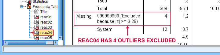 Under Missing we see the number of excluded outliers but not the exact values.
Sadly, we're no longer able to tell precisely which original values these correspond to.
Final Notes
Thus far, I deliberately avoided the discussion precisely which values should be considered outliers for our data. I feel that simply making a decision and being fully explicit about it is more constructive than endless debate.
I therefore blindly followed some rules of thumb for the boxplot and z-score approaches. As I warned earlier, these don't always result in good decisions: for the data at hand, reaction times below some 500 ms can't be taken seriously. However, the rules of thumb don't always exclude these.
As for most of data analysis, using common sense is usually a better idea...
Thanks for reading!
THIS TUTORIAL HAS 25 COMMENTS:
By Peck on October 1st, 2024
Grammatical mishap: I was referring to the SPSS command DETECT ANOMALY. It's not an extension. It is built in.
From the help...
The Anomaly Detection procedure searches for unusual cases based on deviations from the norms of their cluster groups. The procedure is designed to quickly detect unusual cases for data-auditing purposes in the exploratory data analysis step, prior to any inferential data analysis.
The procedure produces peer groups, peer group norms for continuous and categorical variables, anomaly indices based on deviations from peer group norms, and variable impact values for variables that most contribute to a case being considered unusual.
This procedure works with both continuous and categorical variables.
(same email address - it's just a forwarding address)
By Ruben Geert van den Berg on October 1st, 2024
Ah, I see. The one under Identify Unusual Cases.
Interesting that it can handle categorical variables but is there any academic literature or consensus on the underlying algorithms?
Because if not, than my Bachelor/Master students won't be allowed to use it because, well, it's not "academic" enough.
P.s. by "continuous" you mean quantitative, right? Those are fundamentally different things and I don't see any justification for using these terms as if they're interchangeable (even though many people do so anyway).
By Peck on October 1st, 2024
The Algorithms manual has a detailed explanation of what DETECT ANOMALY does, but since it uses TWOSTEP CLUSTER, it refers the reader to that section for references and some details.
However, since this is really an exploratory method - just as univariate detection is, I don't think it needs a detailed justification just as you said in your article conclusion.
By Ruben Geert van den Berg on October 2nd, 2024
Yes and no.
The final question is which cases/values to exclude or remove from the data before analysis.
This decision needs a strong and clear justification and it needs to be transparent.
So my experience with academic environments is that they tend towards z-scores or boxplots because these have fairly clear ("objective") rules for what to exclude.
However, one of my recent videos (I think it was boxplots) clearly showed that such rules may fail completely.
So that's one of the reasons I prefer histograms but these are obviously not objective so they create room to steer outcomes into some desired direction.
IMHO, this really is a difficult grey area.
Statistics is not an exact science and it neither can nor should be.
By Peck on October 2nd, 2024
The Algorithms doc for DETECT ANOMALY and TWOSTEP has all the details, but it would be hard to summarize concisely. Although there is no truly right answer for clustering, this procedure at least has the virtue of being reasonably objective. And one generally doesn't know what caused an outlier, so being objective may be the best you can do.
As an alternative, one might use robust/nonparametric methods, but that, too, is a judgment call.