• Quick Data Screening
• SPSS Split-Half Reliability Dialogs
• SPSS Split-Half Reliability Output
• Spearman-Brown & Horst Formulas
• Specifying our Test Halves

A psychologist is developing a scale to measure “emotional stability”. She therefore adminstered her 15 items to a sample of N = 924 students. The data thus obtained are in split-half-reliability.sav, partly shown below.

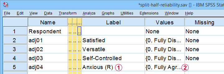
Note that some items indicating emotional instability have been reverse coded. These items have (R) appended to their variable label and their value labels have been adjusted as well.

Now, test reliability is usually examined using Cronbach’s alpha. However, some researchers prefer split-half reliability:

• the items are divided over two test halves;
• the sum scores over the items in each half are computed;
• the Pearson correlation between these 2 sum scores is computed;
• this correlation is adjusted for test length and reported.

So how to find split-half reliability in SPSS? We'll show you in a minute. But let's first make sure we know what's in our data.

Quick Data Screening

A solid way to screen these data is inspecting frequency distributions and their corresponding bar charts. You'll find these under Analyze Descriptive statistics Frequencies but a faster way is to run the SPSS syntax below.

Data Screening Output

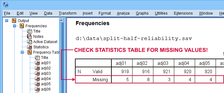
First off, note that the Statistics table indicates that there's some missing values in our variables. Fortunately, they're not too many but they'll have consequences for our analyses nevertheless.

Next up, let's inspect the actual frequency tables. The main question here is whether we should specify any answer categories (such as “No opinion”) as user missing values. Note that these are not present in the data at hand.

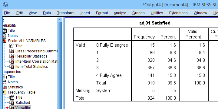
Quick tip: if your tables don't show the actual values (0, 1, ...), then run set tnumbers both tvars both. prior to running your tables as covered in SPSS SET - Quick Tutorial.

Last but not least, scroll through your bar charts like the one shown below.

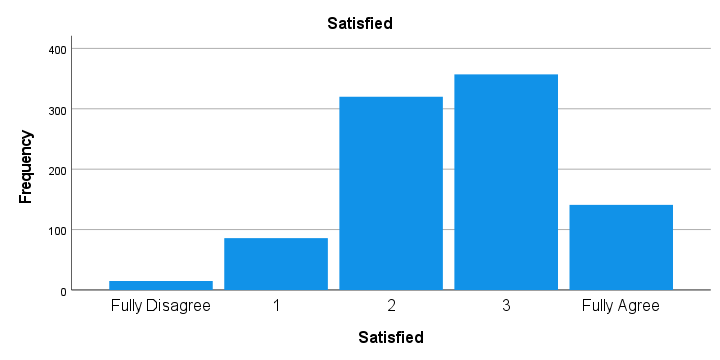
The bar charts for our example data all look perfectly plausible. Most of them have some negative skewness but this makes sense for these data.

So except for a couple of missing values, our data look fine. We can now analyze them with confidence.

SPSS Split-Half Reliability Dialogs

We'll first navigate to Analyze Scale Reliability Analysis and fill out the dialogs as shown below.

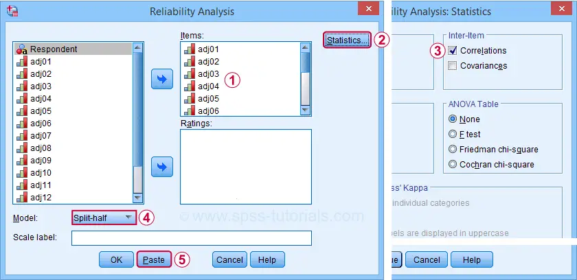
Completing these steps results in the syntax below. Let's run it.

SPSS Split-Half Reliability Output

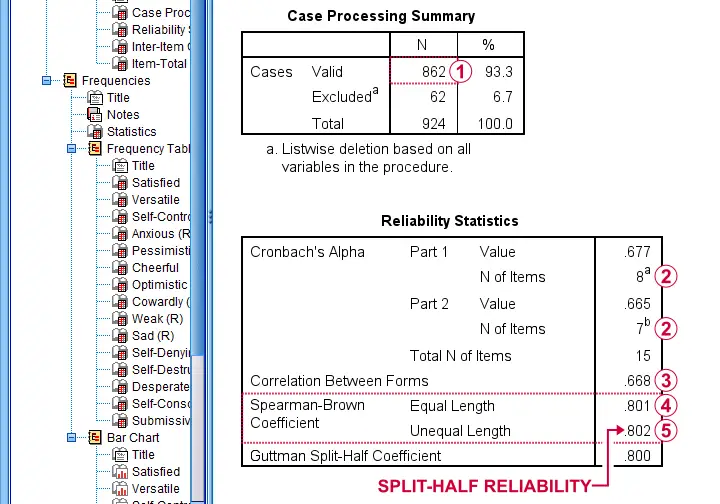
First off, note that this analysis is based on N = 862 out of 924 observations due to missing values.

Next, SPSS defines Part 1 (the first test half) as the first 8 items. As seen in the footnotes, the last 7 items make up Part 2.

The (unadjusted) correlation between the sum scores over these halves, r = .668.

Adjusting this correlation using the Spearman-Brown formula results in r_sb = .801. We'll explain the what and why for this adjustment in a minute.

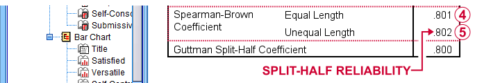
If our test “halves” have unequal lengths, the more appropriate adjustment is the Horst formula⁶ which results in r_h = .802. This is what we report as our split-half reliability.

Note that we also have the correlation matrix among all items in our output. I recommend you quickly scan it for any negative correlations. These don't make sense among items that measure a single trait. So if you do find them, something may be wrong with your data.

For the data at hand, adj12 (Self-Destructive) has some negative correlations. Although they're probably not statistically significant, this item seems rather poor and had perhaps better be removed from our scale.

Quick Replication of Results

Let's now see if we can replicate some of these results. First off, we'll recompute the correlation between the sum scores of our test halves using the syntax below.

This -indeed- yields r = .668. So why and how should this be adjusted?

Spearman-Brown & Horst Formulas

It is well known that test reliability tends to increase with test length^1,7: everything else equal, more items result in higher reliability.

Now, with split-half reliability, we compute the reliability for test halves. And because these are only half as long as the entire test, this greatly attenuates our reliability estimate. So which correlation would we have found for test halves
having the same length as the entire test? This can be estimated by the Spearman-Brown formula, which is

$$r_{sb} = \frac{k \cdot r}{1 + (k - 1) \cdot r}$$

where

• \(r_{sb}\) denotes the Spearman-Brown adjusted correlation;
• \(k\) denotes the factor by which the test length increases and;
• \(r\) denotes unadjusted correlation between test halves.

In this formula,

$$k = \frac{number\;of\; items\; in\; new\; test}{number\;of\; items\; in\; old\; test}$$

For our example, the entire test contains 15 items while our halves have an average length of (8 + 7) / 2 = 7.5 items. Therefore, k = 15 / 7.5 = 2.

That is, our test length increases by a factor 2 (note that this is always the case for split-halves reliability).

Now our Spearman-Brown adjusted correlation is

$$r_{sb} = \frac{2 \cdot 0.668}{1 + (2 - 1) \cdot 0.668} = .801$$

which is precisely what SPSS reports. There's one minor issue, though: the Spearman-Brown formula assumes that the test halves have equal lengths.

If this doesn't hold, Warrens⁶ (2016) argues that the Horst formula should be used instead. In the SPSS output, this is denoted as “Spearman-Brown Coeffient Unequal Length.”

For our example, \(r_h\) = .802 so this is what we report as our split-half reliability.

A minor note here is that the Horst formula simplifies to the Spearman-Brown formula for equal lengths so you can't go wrong by reporting this. Second, Warrens (2016) states that the Horst formula always yields a higher correlation for unequal lengths but the difference tends to be negligible.

Specifying our Test Halves

Now what if we'd like to define our test halves differently? That's fairly simple: for k items, SPSS always uses

• the first k / 2 items as part 1 and all other items as part 2 if k is even;
• the first k / 2 + 0.5 items as part 1 if k is odd.

That is, for 15 items, the first 8 items that you enter are always part 1. All other items are part 2. So if we'd like to use items 1 - 7 as our first half, we simply specify them after items 8 - 15 as shown below.

Right, so that's all folks. I hope you found this tutorial helpful. If you've any questions or remarks, please throw me a comment below.

Thanks for reading!

References

1. Drenth, P. & Sijtsma, K. (2015) Testtheorie. Inleiding in de Theorie van de Psychologische Test en zijn Toepassingen [Test theory. Introduction to the theory of the Psychological Test and its Applications]. Houten: Bohn Stafleu van Loghum
2. Field, A. (2013). Discovering Statistics with IBM SPSS Statistics. Newbury Park, CA: Sage.
3. Howell, D.C. (2002). Statistical Methods for Psychology (5th ed.). Pacific Grove CA: Duxbury.
4. Pituch, K.A. & Stevens, J.P. (2016). Applied Multivariate Statistics for the Social Sciences (6th. Edition). New York: Routledge.
5. Warner, R.M. (2013). Applied Statistics (2nd. Edition). Thousand Oaks, CA: SAGE.
6. Warrens, M.J. (2016). A comparison of reliability coefficients for psychometric tests that consist of two parts. Advances in Data Analysis and Classification, 10(1), 71-84.
7. Van den Brink, W.P. & Mellenberg, G.J. (1998). Testleer en testconstructie [Test science and test construction]. Amsterdam: Boom.