• Z-Test - Assumptions
• SPSS Z-Tests Dialogs
• SPSS Z-Test Output
• SPSS Z-Tests - Strengths & Weaknesses
• APA Reporting Z-Tests

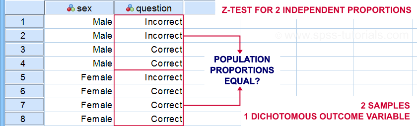
A z-test for independent proportions tests if 2 subpopulations
score similarly on a dichotomous variable. Example: are the proportions (or percentages) of correct answers equal between male and female students?

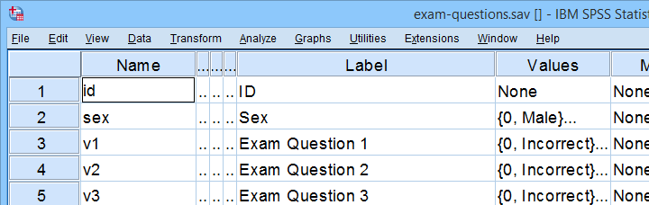
Although z-tests are widely used in the social sciences, they were only introduced in SPSS version 27. So let's see how to run them and interpret their output. We'll use exam-questions.sav -partly shown below- throughout this tutorial.

Now, before running the actual z-tests, we first need to make sure we meet their assumptions.

Z-Test - Assumptions

Z-tests for independent proportions require 2 assumptions:

• independent observations and
• sufficient sample sizes.

Regarding this second assumption, Agresti and Franklin (2014)² propose that both outcomes should occur at least 10 times in both samples. That is,

$$p_a n_a \ge 10, (1 - p_a) n_a \ge 10, p_b n_b \ge 10, (1 - p_b) n_b \ge 10$$

where

• \(n_a\) and \(n_b\) denote the sample sizes of groups a and b and
• \(p_a\) and \(p_b\) denote the proportions of “successes” in both groups.

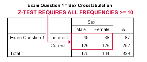
Note that some other textbooks^3,4 suggest that smaller sample sizes may be sufficient. If you're not sure about meeting the sample sizes assumption, run a minimal CROSSTABS command as in crosstabs v1 to v5 by sex. As shown below, note that all 5 exam questions easily meet the sample sizes assumption.

For insufficient sample sizes, Agresti and Caffo (2000)¹ proposed a simple adjustment for computing confidence intervals: simply add one observation for each outcome to each group (4 observations in total) and proceed as usual with these adjusted sample sizes.

SPSS Z-Tests Dialogs

First off, let's navigate to Analyze Compare Means Independent-Samples Proportions and fill out the dialogs as shown below.

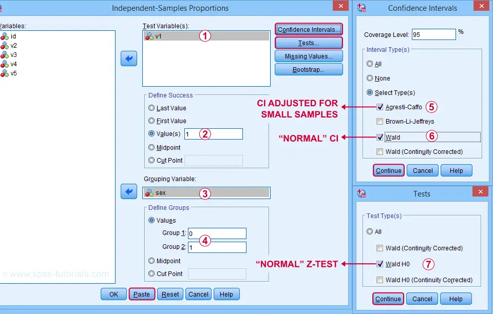
Clicking “Paste” results in the SPSS syntax below. Let's run it.

SPSS Z-Test Output

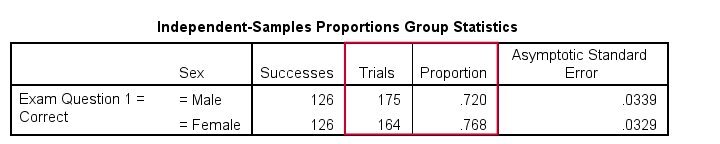
The first table shows the observed proportions for male and female students. Note that female students seem to perform somewhat better: a proportion of .768 (or 76.8%) answered correctly as compared to .720 for male students.

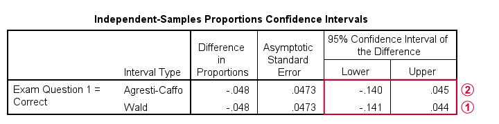
The second output table shows that the difference between our sample proportions is -.048.

The “normal” 95% confidence interval for this difference (denoted as Wald) is [-.141, .044]. Note that this CI encloses zero: male and female populations performing equally well is within the range of likely values.

I don't recommend reporting the Agresti-Caffo corrected CI unless your data don't meet the sample sizes assumption.

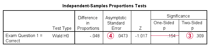
The third table shows the z-test results. First note that p(2-tailed) = .309. As a rule of thumb, we reject the null hypothesis if p < 0.05 which is not the case here. Conclusion: we do not reject the null hypothesis that the population difference is zero. That is: the sample difference of -.048 is not statistically significant.

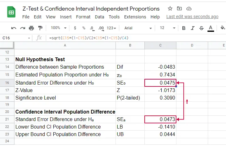
Finally, note that SPSS reports the wrong standard error for this test. The correct standard error is 0.0475 as computed in this Googlesheet (read-only) shown below.

SPSS Z-Tests - Strengths and Weaknesses

What's good about z-tests in SPSS is that

• you can analyze many dependent variables in one go;
• both the independent and dependent variables may be either string variables or numeric variables;We also tested SPSS z-tests on a mixture of string and numeric dependent variables. Although doing so is very awkward, the results were correct.
• many corrections -such as Agresti-Caffo- are available.

However, what I really don't like about SPSS z-tests is that

• no warning is issued if the sample sizes assumption isn't met;
• no effect size measures are available. Cohen’s H seems completely absent from SPSS and phi coefficients are available from CROSSTABS or CORRELATIONS;
• SPSS reports the wrong standard error for the actual z-test;
• z-tests and confidence intervals are reported in separate tables. I'd rather see these as different columns in a single table with one row per dependent variable.

APA Reporting Z-Tests

The APA guidelines don't explicitly mention how to report z-tests. However, it makes sense to report something like the difference between males and females
was not significant, z = -1.02, p(2-tailed) = .309. You should obviously report the actual proportions and sample sizes as well. If you analyzed multiple dependent variables, you may want to create a table showing

• both proportions being compared;
• the difference between the proportions and its confidence interval;
• z and p(2-tailed) for the null hypothesis of equal population proportions;
• some effect size measure.

References

1. Agresti, A & Caffo, B. (2000). Simple and Effective Confidence Intervals for Proportions and Differences of Proportions. The American Statistician, 54(4), 280-288.
2. Agresti, A. & Franklin, C. (2014). Statistics. The Art & Science of Learning from Data. Essex: Pearson Education Limited.
3. Twisk, J.W.R. (2016). Inleiding in de Toegepaste Biostatistiek [Introduction to Applied Biostatistics]. Houten: Bohn Stafleu van Loghum.
4. Van den Brink, W.P. & Koele, P. (2002). Statistiek, deel 3 [Statistics, part 3]. Amsterdam: Boom.