There's two basic tests for testing a single proportion:
- the binomial test and
- the z-test for a single proportion.
For larger samples, these tests result in roughly similar p-values. However, the binomial test only comes up with a 1-tailed p-value unless the hypothesized proportion = 0.5. Moreover, it can't compute a confidence interval for your proportion.
The z-test does not have these 2 limitations and is among the more widely used statistical tests. Very oddly, however, it's absent from SPSS. Plenty of reasons for us to present this very simple tool in the remainder of this tutorial.
Installation
- This tool requires SPSS version 18 or higher with the SPSS Python Essentials properly installed and tested.
- Download the Confidence Interval Proportion tool.
- For SPSS versions 18 through 22, select
 . For SPSS 24, select .
Navigate to the confidence intervals extension (its file name ends in “.spe”, short for SPSS Extension) and install it. - Although you'll get a popup that the extension was successfully installed, it'll only work after you close and reopen SPSS entirely (unless you're on version 24).
- You'll now find the tool under .
Operations
- The test variables must have exactly two valid values. Variables violating this requirement will be skipped when calculating results.
- The test variables may be any mixture of numeric and string variables.
- The p-values and confidence intervals are based on the central limit theorem. This approximation is sufficiently accurate if p0*n and (1-p0)*n >5 where p0 denotes the population proportion under H0 and n is its related sample size.1 If this does not hold for one or more variables, a note will be added to the results.
- If any SPLIT FILE is in effect, the tool will switch if off, throw a warning that it did so and then proceed as usual.
- If a WEIGHT variable is in effect, results will be based on rounded frequencies. P-values may be biased if you're using non integer sampling weights but this holds for all p-values in SPSS except for those from the complex samples module.2,3,4
Example
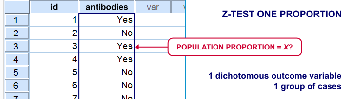
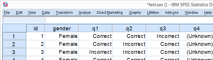
We'll now test our tool on test.sav, part of which is shown below. Our null hypothesis is that the population proportions of all dichotomous variables = 0.5.
Data Inspection
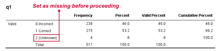
We'll run a quick data check with FREQUENCIES to see if we need to specify any user missing values. This happens to be the case so we'll do just that.
set tnumbers both.
*Basic frequency tables.
frequencies q1 to passes.
*Set missing values.
missing values q1 to q4 (2).
*Show only value labels in output.
set tnumbers labels.
Result
Computing our Confidence Intervals
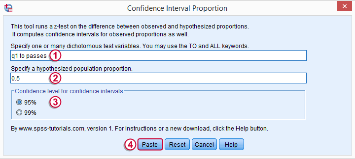
We'll go to ![]() and fill out the main dialog as below.
and fill out the main dialog as below.
 Note that TO may be used for a range of variable names.
 Clicking results in the syntax below.
CONFIDENCE_INTERVAL_PROPORTION VARIABLES = 'q1 to passes' TESTPROP = 0.5 LEVEL = 95.
Results
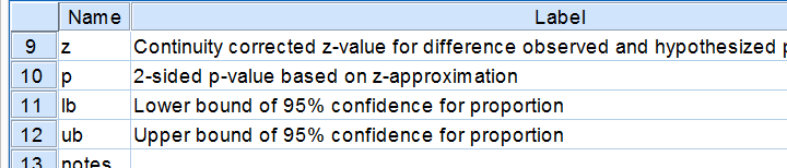
Running our syntax results in a new dataset holding our results. Note that most variables have variable labels explaining their precise meaning. You can see them in variable view or hover over a variable’s name in data view as shown in the screenshot below.
We find back our (valid) frequencies in these results. Each test variable has in 2 rows, one for each value. You'll probably need just one of these rows but this configuration circumvents the need for specifying test values for each variable. We simply test both -whatever they may be.
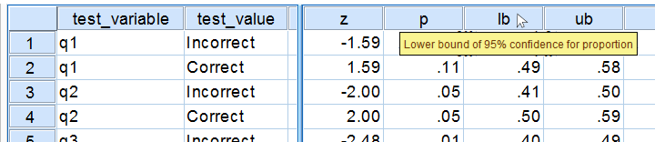
Further right we find our z-test. Its p-value indicates the probability of finding the observed sample proportions if its population counterpart is exactly equal to the test proportion. Note that a continuity correction has been used for computing the z-values and their associated p-values. Finally, the last variables in our results hold our confidence intervals and -possibly- some notes on the results.
Reporting Examples
Obviously, include your sample proportions and sample size in your report. Regarding the z-tests, we'll write something like “the proportion of people who answered q1 correctly did not differ from 0.5, as indicated by a z-test: z = 1.59, p = 0.11.”or “A z-test showed that more than 50% of our population answers q2 correctly, z = 2.0, p = 0.046.”
Thanks for reading, hope you'll like it!
References
- Van den Brink, W.P. & Koele, P. (2002). Statistiek, deel 3 [Statistics, part 3]. Amsterdam: Boom.
- Fowler, F.J. (2009). Survey Research Methods. Thousand Oaks, CA: SAGE.
- De Leeuw, E.D., Hox, J.J. and Dillman, D.A. (2008). International Handbook of Survey Methodology. New York: Lawrence Erlbaum Associates.
- Kish, L. Weighting for Unequal Pi. Journal of Official Statistics, 8, 183-200.
THIS TUTORIAL HAS 16 COMMENTS:
By Ruben Geert van den Berg on October 23rd, 2022
Note that z-tests only apply to dichotomous variables -that is, variables having precisely 2 (valid) values.
If you've more than 2 distinct values, you can dichotomize these. Likely options for this are RECODE and/or IF.
Hope that helps!
SPSS tutorials