Logistic Regression – Simple Introduction

• Logistic Regression Equation
• Logistic Regression Example Curves
• Logistic Regression - B-Coefficients
• Logistic Regression - Effect Size
• Logistic Regression Assumptions

Logistic regression is a technique for predicting a
dichotomous outcome variable from 1+ predictors. Example: how likely are people to die before 2020, given their age in 2015? Note that “die” is a dichotomous variable because it has only 2 possible outcomes (yes or no).

This analysis is also known as binary logistic regression or simply “logistic regression”. A related technique is multinomial logistic regression which predicts outcome variables with 3+ categories.

Logistic Regression - Simple Example

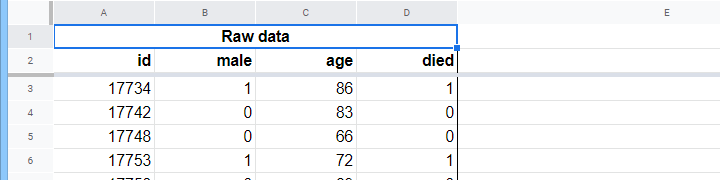
A nursing home has data on N = 284 clients’ sex, age on 1 January 2015 and whether the client passed away before 1 January 2020. The raw data are in this Googlesheet, partly shown below.

Let's first just focus on age: can we predict death before 2020 from age in 2015? And -if so- precisely how? And to what extent? A good first step is inspecting a scatterplot like the one shown below.

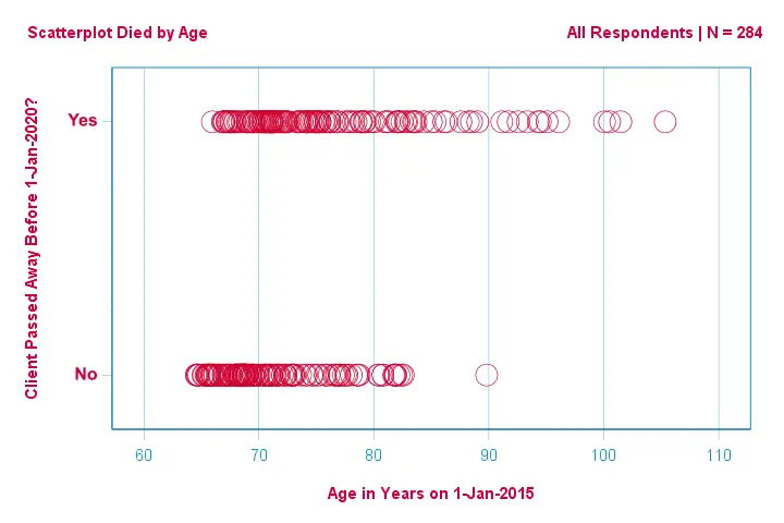
A few things we see in this scatterplot are that

• all but one client over 83 years of age died within the next 5 years;
• the standard deviation of age is much larger for clients who died than for clients who survived;
• age has a considerable positive skewness, especially for the clients who died.

But how can we predict whether a client died, given his age? We'll do just that by fitting a logistic curve.

Simple Logistic Regression Equation

Simple logistic regression computes the probability of some outcome given a single predictor variable as

$$P(Y_i) = \frac{1}{1 + e^{\,-\,(b_0\,+\,b_1X_{1i})}}$$

where

• \(P(Y_i)\) is the predicted probability that \(Y\) is true for case \(i\);
• \(e\) is a mathematical constant of roughly 2.72;
• \(b_0\) is a constant estimated from the data;
• \(b_1\) is a b-coefficient estimated from the data;
• \(X_i\) is the observed score on variable \(X\) for case \(i\).

The very essence of logistic regression is estimating \(b_0\) and \(b_1\). These 2 numbers allow us to compute the probability of a client dying given any observed age. We'll illustrate this with some example curves that we added to the previous scatterplot.

Logistic Regression Example Curves

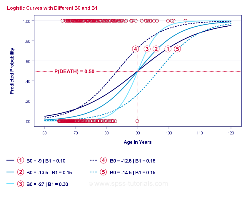
If you take a minute to compare these curves, you may see the following:

• \(b_0\) determines the horizontal position of the curves: as \(b_0\) increases, the curves shift towards the left but their steepnesses are unaffected. This is seen for curves , and . Note that \(b_0\) is different but \(b_1\) is equal for these curves.
• As \(b_0\) increases, predicted probabilities increase as well: given age = 90 years, curve predicts a roughly 0.75 probability of dying. Curves and predict roughly 0.50 and 0.25 probabilities of dying for a 90-year old client.
• \(b_1\) determines the steepness of the curves: if \(b_1\) > 0, the probability of dying increases with increasing age. This relation becomes stronger as \(b_1\) becomes larger. Curves , and illustrate this point: as \(b_1\) becomes larger, the curves get steeper so the probability of dying increases faster with increasing age.

For now, we've one question left: how do we find the “best” \(b_0\) and \(b_1\)?

Logistic Regression - Log Likelihood

For each respondent, a logistic regression model estimates the probability that some event \(Y_i\) occurred. Obviously, these probabilities should be high if the event actually occurred and reversely. One way to summarize how well some model performs for all respondents is the log-likelihood \(LL\):

$$LL = \sum_{i = 1}^N Y_i \cdot ln(P(Y_i)) + (1 - Y_i) \cdot ln(1 - P(Y_i))$$

where

• \(Y_i\) is 1 if the event occurred and 0 if it didn't;
• \(ln\) denotes the natural logarithm: to what power must you raise \(e\) to obtain a given number?

\(LL\) is a goodness-of-fit measure: everything else equal, a logistic regression model fits the data better insofar as \(LL\) is larger. Somewhat confusingly, \(LL\) is always negative. So we want to find the \(b_0\) and \(b_1\) for which
\(LL\) is as close to zero as possible.

Maximum Likelihood Estimation

In contrast to linear regression, logistic regression can't readily compute the optimal values for \(b_0\) and \(b_1\). Instead, we need to try different numbers until \(LL\) does not increase any further. Each such attempt is known as an iteration. The process of finding optimal values through such iterations is known as maximum likelihood estimation.

So that's basically how statistical software -such as SPSS, Stata or SAS- obtain logistic regression results. Fortunately, they're amazingly good at it. But instead of reporting \(LL\), these packages report \(-2LL\). \(-2LL\) is a “badness-of-fit” measure which follows a
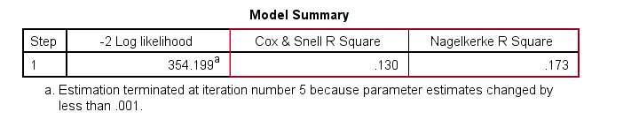
chi-square-distribution. This makes \(-2LL\) useful for comparing different models as we'll see shortly. \(-2LL\) is denoted as -2 Log likelihood in the output shown below.

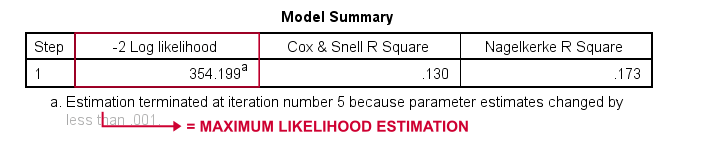
The footnote here tells us that the maximum likelihood estimation needed only 5 iterations for finding the optimal b-coefficients \(b_0\) and \(b_1\). So let's look into those now.

Logistic Regression - B-Coefficients

The most important output for any logistic regression analysis are the b-coefficients. The figure below shows them for our example data.

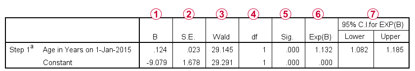
Before going into details, this output briefly shows

the b-coefficients that make up our model;
the standard errors for these b-coefficients;
the Wald statistic -computed as \((\frac{B}{SE})^2\)- which follows a chi-square distribution;
the degrees of freedom for the Wald statistic;
the significance levels for the b-coefficients;
exponentiated b-coefficients or \(e^B\) are the odds ratios associated with changes in predictor scores;
the 95% confidence interval for the exponentiated b-coefficients.

The b-coefficients complete our logistic regression model, which is now

$$P(death_i) = \frac{1}{1 + e^{\,-\,(-9.079\,+\,0.124\, \cdot\, age_i)}}$$

For a 75-year-old client, the probability of passing away within 5 years is

$$P(death_i) = \frac{1}{1 + e^{\,-\,(-9.079\,+\,0.124\, \cdot\, 75)}}=$$

$$P(death_i) = \frac{1}{1 + e^{\,-\,0.249}}=$$

$$P(death_i) = \frac{1}{1 + 0.780}=$$

$$P(death_i) \approx 0.562$$

So now we know how to predict death within 5 years given somebody’s age. But how good is this prediction? There's several approaches. Let's start off with model comparisons.

Logistic Regression - Baseline Model

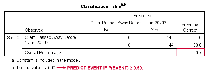
How could we predict who passed away if we didn't have any other information? Well, 50.7% of our sample passed away. So the predicted probability would simply be 0.507 for everybody.

For classification purposes, we usually predict that an event occurs if p(event) ≥ 0.50. Since p(died) = 0.507 for everybody, we simply predict that everybody passed away. This prediction is correct for the 50.7% of our sample that died.

Logistic Regression - Likelihood Ratio

Now, from these predicted probabilities and the observed outcomes we can compute our badness-of-fit measure: -2LL = 393.65. Our actual model -predicting death from age- comes up with -2LL = 354.20. The difference between these numbers is known as the likelihood ratio \(LR\):

$$LR = (-2LL_{baseline}) - (-2LL_{model})$$

Importantly, \(LR\) follows a chi-square distribution with \(df\) degrees of freedom, computed as

$$df = k_{model} - k_{baseline}$$

where \(k\) denotes the numbers of parameters estimated by the models. As shown in this Googlesheet, \(LR\) and \(df\) result in a significance level for the entire model.

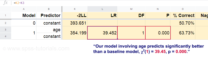
The null hypothesis here is that some model predicts equally poorly as the baseline model in some population. Since p = 0.000, we reject this: our model (predicting death from age) performs significantly better than a baseline model without any predictors.
But precisely how much better? This is answered by its effect size.

Logistic Regression - Model Effect Size

A good way to evaluate how well our model performs is from an effect size measure. One option is the Cox & Snell R² or \(R^2_{CS}\) computed as

$$R^2_{CS} = 1 - e^{\frac{(-2LL_{model})\,-\,(-2LL_{baseline})}{n}}$$

Sadly, \(R^2_{CS}\) never reaches its theoretical maximum of 1. Therefore, an adjusted version known as Nagelkerke R² or \(R^2_{N}\) is often preferred:

$$R^2_{N} = \frac{R^2_{CS}}{1 - e^{-\frac{-2LL_{baseline}}{n}}}$$

For our example data, \(R^2_{CS}\) = 0.130 which indicates a medium effect size. \(R^2_{N}\) = 0.173, slightly larger than medium.

Last, \(R^2_{CS}\) and \(R^2_{N}\) are technically completely different from r-square as computed in linear regression. However, they do attempt to fulfill the same role. Both measures are therefore known as pseudo r-square measures.

Logistic Regression - Predictor Effect Size

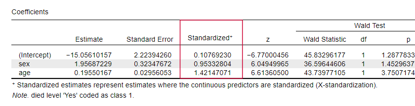
Oddly, very few textbooks mention any effect size for individual predictors. Perhaps that's because these are completely absent from SPSS. The reason we do need them is that b-coefficients depend on the (arbitrary) scales of our predictors: if we'd enter age in days instead of years, its b-coefficient would shrink tremendously. This obviously renders b-coefficients unsuitable for comparing predictors within or across different models.
JASP includes partially standardized b-coefficients: quantitative predictors -but not the outcome variable- are entered as z-scores as shown below.

Logistic Regression Assumptions

Logistic regression analysis requires the following assumptions:

1. independent observations;
2. correct model specification;
3. errorless measurement of outcome variable and all predictors;
4. linearity: each predictor is related linearly to \(e^B\) (the odds ratio).

Assumption 4 is somewhat disputable and omitted by many textbooks^1,6. It can be evaluated with the Box-Tidwell test as discussed by Field⁴. This basically comes down to testing if there's any interaction effects between each predictor and its natural logarithm or \(LN\).

Multiple Logistic Regression

Thus far, our discussion was limited to simple logistic regression which uses only one predictor. The model is easily extended with additional predictors, resulting in multiple logistic regression:

$$P(Y_i) = \frac{1}{1 + e^{\,-\,(b_0\,+\,b_1X_{1i}+\,b_2X_{2i}+\,...+\,b_kX_{ki})}}$$

where

• \(P(Y_i)\) is the predicted probability that \(Y\) is true for case \(i\);
• \(e\) is a mathematical constant of roughly 2.72;
• \(b_0\) is a constant estimated from the data;
• \(b_1\), \(b_2\), ... ,\(b_k\) are the b-coefficient for predictors 1, 2, ... ,\(k\);
• \(X_{1i}\), \(X_{2i}\), ... ,\(X_{ki}\) are observed scores on predictors \(X_1\), \(X_2\), ... ,\(X_k\) for case \(i\).

Multiple logistic regression often involves model selection and checking for multicollinearity. Other than that, it's a fairly straightforward extension of simple logistic regression.

Logistic Regression - Next Steps

This basic introduction was limited to the essentials of logistic regression. If you'd like to learn more, you may want to read up on some of the topics we omitted:

1. odds ratios -computed as \(e^B\) in logistic regression- express how probabilities change depending on predictor scores ;
2. the Box-Tidwell test examines if the relations between the aforementioned odds ratios and predictor scores are linear;
3. the Hosmer and Lemeshow test is an alternative goodness-of-fit test for an entire logistic regression model.

Thanks for reading!

References

1. Warner, R.M. (2013). Applied Statistics (2nd. Edition). Thousand Oaks, CA: SAGE.
2. Agresti, A. & Franklin, C. (2014). Statistics. The Art & Science of Learning from Data. Essex: Pearson Education Limited.
3. Hair, J.F., Black, W.C., Babin, B.J. et al (2006). Multivariate Data Analysis. New Jersey: Pearson Prentice Hall.
4. Field, A. (2013). Discovering Statistics with IBM SPSS Statistics. Newbury Park, CA: Sage.
5. Howell, D.C. (2002). Statistical Methods for Psychology (5th ed.). Pacific Grove CA: Duxbury.
6. Pituch, K.A. & Stevens, J.P. (2016). Applied Multivariate Statistics for the Social Sciences (6th. Edition). New York: Routledge.

How to Run Levene’s Test in SPSS?

Levene’s test examines if 2+ populations all have
equal variances on some variable.

• Null Hypothesis
• Assumptions
• Levene’s test in SPSS
• Output
• Reporting

Levene’s Test - What Is It?

If we want to compare 2(+) groups on a quantitative variable, we usually want to know if they have equal mean scores. For finding out if that's the case, we often use

• an independent samples t-test for comparing 2 groups or
• a one-way ANOVA for comparing 3+ groups.

Both tests require the homogeneity (of variances) assumption: the population variances of the dependent variable must be equal within all groups. However, you don't always need this assumption:

• you don't need to meet the homogeneity assumption if the groups you're comparing have roughly equal sample sizes;
• you do need this assumption if your groups have sharply different sample sizes.

Now, we usually don't know our population variances but we do know our sample variances. And if these don't differ too much, then the population variances being equal seems credible.

But how do we know if our sample variances differ “too much”? Well, Levene’s test tells us precisely that.

Null Hypothesis

The null hypothesis for Levene’s test is that the groups we're comparing all have equal population variances. If this is true, we'll probably find slightly different variances in samples from these populations. However, very different sample variances suggest that the population variances weren't equal after all. In this case we'll reject the null hypothesis of equal population variances.

Levene’s Test - Assumptions

Levene’s test basically requires two assumptions:

• independent observations and
• the test variable is quantitative -that is, not nominal or ordinal.

Levene’s Test - Example

A fitness company wants to know if 2 supplements for stimulating body fat loss actually work. They test 2 supplements (a cortisol blocker and a thyroid booster) on 20 people each. An additional 40 people receive a placebo.

All 80 participants have body fat measurements at the start of the experiment (week 11) and weeks 14, 17 and 20. This results in fatloss-unequal.sav, part of which is shown below.

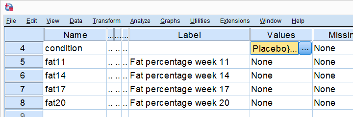
One approach to these data is comparing body fat percentages over the 3 groups (placebo, thyroid, cortisol) for each week separately.Perhaps a better approach to these data is using a single mixed ANOVA. Weeks would be the within-subjects factor and supplement would be the between-subjects factor. For now, we'll leave it as an exercise to the reader to carry this out. This can be done with an ANOVA for each of the 4 body fat measurements. However, since we've unequal sample sizes, we first need to make sure that our supplement groups have equal variances.

Running Levene’s test in SPSS

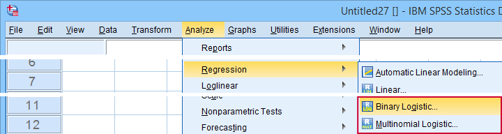
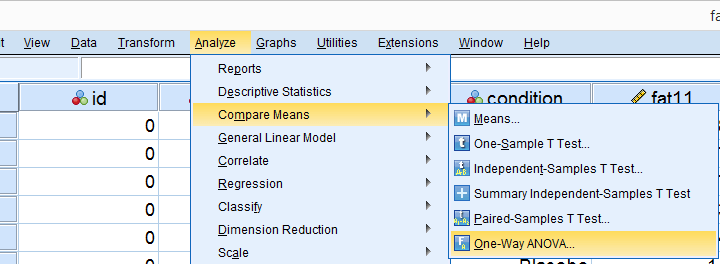
Several SPSS commands contain an option for running Levene’s test. The easiest way to go -especially for multiple variables- is the One-Way ANOVA dialog.This dialog was greatly improved in SPSS version 27 and now includes measures of effect size such as (partial) eta squared. So let's navigate to Analyze Compare Means One-Way ANOVA and fill out the dialog that pops up.

As shown below, the Homogeneity of variance test under Options refers to Levene’s test.

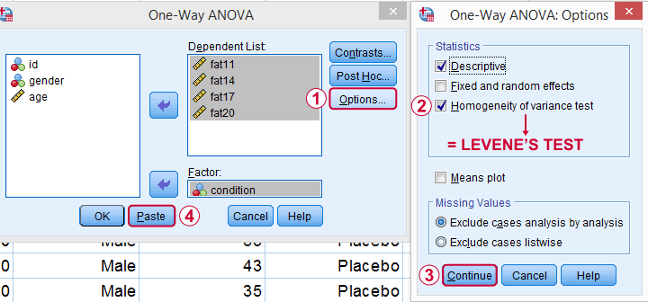
Clicking Paste results in the syntax below. Let's run it.

SPSS Levene’s Test Syntax Example

Output for Levene’s test

On running our syntax, we get several tables. The second -shown below- is the Test of Homogeneity of Variances. This holds the results of Levene’s test.

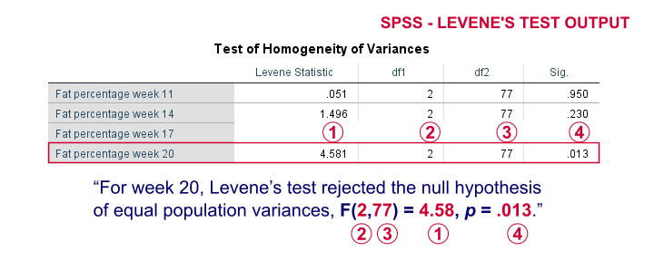
As a rule of thumb, we conclude that population variances are not equal if “Sig.” or p < .05. For the first 2 variables, p > .05: for fat percentage in weeks 11 and 14 we don't reject the null hypothesis of equal population variances.

For the last 2 variables, p < .05: for fat percentages in weeks 17 and 20, we reject the null hypothesis of equal population variances. So these 2 variables violate the homogeneity of variance assumption needed for an ANOVA.

Descriptive Statistics Output

Remember that we don't need equal population variances if we have roughly equal sample sizes. A sound way for evaluating if this holds is inspecting the Descriptives table in our output.

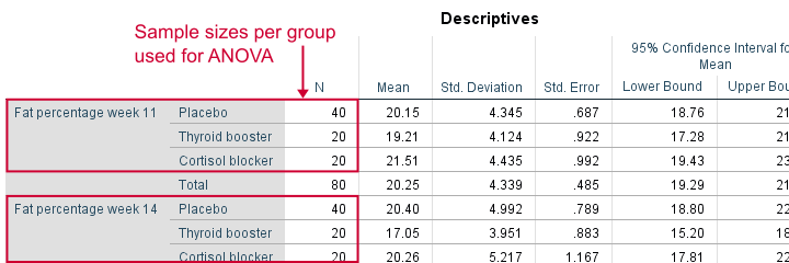
As we see, our ANOVA is based on sample sizes of 40, 20 and 20 for all 4 dependent variables. Because they're not (roughly) equal, we do need the homogeneity of variance assumption but it's not met by 2 variables.

In this case, we'll report alternative measures (Welch and Games-Howell) that don't require the homogeneity assumption. How to run and interpret these is covered in SPSS ANOVA - Levene’s Test “Significant”.

Reporting Levene’s test

Perhaps surprisingly, Levene’s test is technically an ANOVA as we'll explain here. We therefore report it like just a basic ANOVA too. So we'll write something like “Levene’s test showed that the variances for body fat percentage in week 20 were not equal, F(2,77) = 4.58, p = .013.”

Levene’s Test - How Does It Work?

Levene’s test works very simply: a larger variance means that -on average- the data values are “further away” from their mean. The figure below illustrates this: watch the histograms become “wider” as the variances increase.

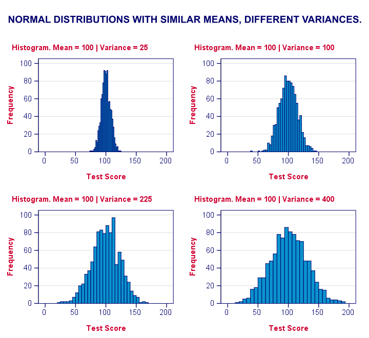
We therefore compute the absolute differences between all scores and their (group) means. The means of these absolute differences should be roughly equal over groups. So technically, Levene’s test is an ANOVA on the absolute difference scores. In other words: we run an ANOVA (on absolute differences) to find out if we can run an ANOVA (on our actual data).

If that confuses you, try running the syntax below. It does exactly what I just explained.

“Manual” Levene’s Test Syntax

Result

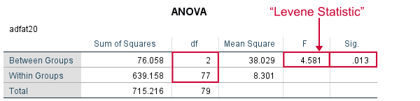
As we see, these ANOVA results are identical to Levene’s test in the previous output. I hope this clarifies why we report it as an ANOVA as well.

Thanks for reading!