How to Draw A Stratified Random Sample in SPSS?
“I have 5 groups of 10 cases in my data. How can I draw a stratified random sample from these cases? That is, from groups 1 through 5 I'd like to draw exactly 5, 4, 5, 6 and 3 cases at random. What's an efficient way to do this?”
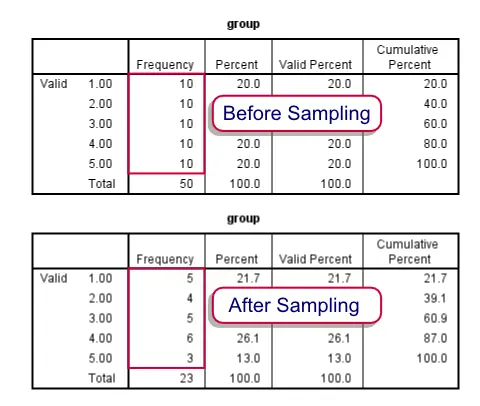 Before and after drawing our stratified sample
Summary
We'll first just demonstrate how to draw the desired sample. After doing so we'll explain in more detail how it works. Unlike the test data we're using here, groups are likely to be defined by more than a single variable. We propose you combine these into a single group variable as described in Combine Categorical Variables. This is not strictly necessary but greatly facilitates the procedure.
Note that the first block of syntax below simply creates a small dataset for demonstrational purposes. We recommend you just run and otherwise ignore it. The actual solution starts in step 3.
SPSS Syntax Example
set seed 1.
input program.
loop group = 1 to 5.
leave group.
loop #cases_per_group = 1 to 10.
end case.
end loop.
end loop.
end file.
end input program.
exe.
*2. Confirm that each group holds 10 cases.
freq group.
*3. Compute completely random variable.
compute random = rv.uniform(0,1).
exe.
*4. Rank random variable within each group.
rank random by group.
*5. Delete 'unsampled' cases from each group.
do repeat current_group = 1 to 5 / desired_freq = 5 4 5 6 3.
select if group ne current_group or rrandom le desired_freq.
end repeat.
*6. Confirm that remaining cases per group are as desired.
frequencies group.
*7. Delete temporary helper variables.
delete variables random rrandom.
SPSS Syntax Steps 3 and 4
The basic trick here is to first COMPUTE a completely random variable. One option for doing so is
COMPUTE random = RV.UNIFORM(0,1).
Depending on your system settings you'll probably see 2 decimals. However, it has many more. You can make them visible by running (for instance) FORMATS random (f6.5). The large number of decimals practically ensures that no ties will occur, which would complicate the approach we're taking here. Next, RANK rrandom BY group. basically results in a counter variable for (randomly sorted) cases within groups.
SPSS Syntax Step 5
Note that at this point it is very easy to draw a fixed number of cases from each group with SELECT IF. For example,SELECT IF rrandom LE 5.will leave a random sample of 5 cases in each group. However, we'd like different numbers of cases from different groups. We can accomplish this with a SELECT IF statement for each group separately. For exampleSELECT IF group NE 1 or rrandom LE 5. deletes all cases from group 1 that have rrandom GT 5. This leaves a random sample of exactly 5 cases in group 1, which we confirm with FREQUENCIES.
Since we'd like such a SELECT IF command for each of our groups, we can shorten our code by wrapping it in a DO REPEAT command.
Sampling in SPSS – Quick Tutorial
How to draw one or many samples from your data in SPSS? This tutorial demonstrates some simple ways for doing so. We'll point out some tips, tricks and pitfalls along the way.
Let's get started and create some test data by running the syntax below.
SPSS Syntax for Creating Test Data
data list free/id.
begin data
0 0 0 0 0 0 0 0 0 0 0 0 0 0 0 0 0 0 0 0 0 0 0 0 0 0 0 0 0 0 0 0 0 0 0 0 0 0 0 0 0 0 0 0 0 0 0 0 0 0
0 0 0 0 0 0 0 0 0 0 0 0 0 0 0 0 0 0 0 0 0 0 0 0 0 0 0 0 0 0 0 0 0 0 0 0 0 0 0 0 0 0 0 0 0 0 0 0 0 0
end data.
compute id = $casenum.
execute.
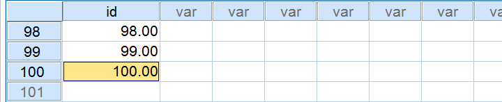
Result
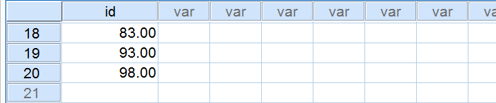
We now have 1 variable and 100 cases. For each case, our variable contains $casenum. The screenshot below shows the last handful of cases in our data.
Simple Sampling Without Replacement
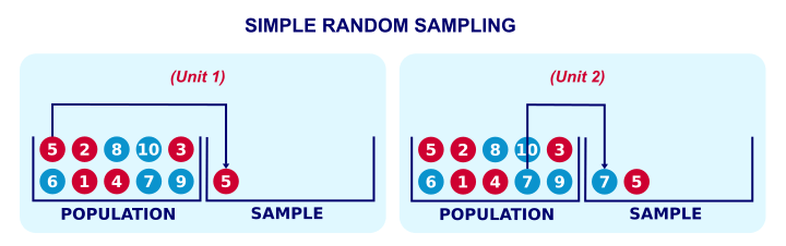
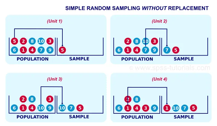
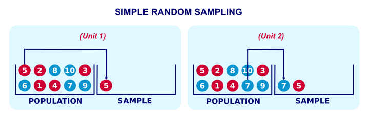
Simple random sampling means that each unit in our population has the same probability of being sampled. “Without replacement” means that a sampled unit is not replaced into the population and thus can be sampled only once. The figure below illustrates the process.
Simple random sampling without replacement is the easiest option for sampling in SPSS. The syntax below shows the first option for doing so.
Simple Random Sampling without Replacement - Example I
set rng mc seed 1.
*2. Draw sample.
sample 20 from 100.
execute.
Result
Notes
This first example is the easiest way to draw just one sample when we know the number of cases in our data (100 in our example). Note that we have 20 cases left after running it.
If we rerun our sampling syntax, we usually want the exact same random sample to come up. One way for ensuring this is running
SET RNG MC SEED 1.
just prior to sampling.
Simple Random Sampling without Replacement - Example II
Let's first rerun our test data syntax. Next, the syntax below shows a second option for sampling without replacement.
compute s1 = rv.uniform(0,1).
*2. Rank random numbers.
rank s1.
*3. Select 20 cases with lowest random numbers.
select if (rs1 <= 20).
execute.
Notes
As we'll see later on, this second example is a first step towards repeated sampling and stratified random sampling. On top, it doesn't require knowing how many cases we have in our data.
Simple Random Sampling without Replacement - Example III
Again, we'll rerun our test data syntax, followed by the syntax below.
set seed 1.
compute s1 = rv.uniform(0,1).
*2. Rank random numbers.
rank s1.
*3. Recode rank variable into filter variable.
recode rs1 (lo thru 20 = 1)(else = 0).
*4. Switch filter on.
filter by rs1.
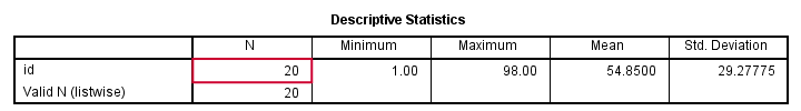
*5. Inspect output.
descriptives id.
Result
Notes
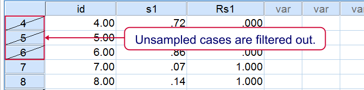
This third examples uses FILTER instead of deleting unsampled cases with SELECT IF. This leaves all our cases -including a variable that indicates our sample- nicely intact in our data. As shown below, the strikethrough in data view as well as the status bar tell us that a filter is actually in effect.
Repetitive Sampling in SPSS
Repeated random sampling is the basis for most simulation studies. We presented such simulations for explaining the basic idea behind ANOVA and the chi-square test.
Simulation studies usually require looping over SPSS procedures, which are basically commands that inspect all cases in our dataset. The right way for doing so is with Python as shown in the syntax below. Running it requires the SPSS Python Essentials to be properly installed.
SPSS Repeated Sampling with Python Syntax
begin program.
import spss
for sample in range(10):
spss.Submit('''
temporary.
sample 20 from 100.
descriptives id.
''')
end program.
Notes
We use TEMPORARY here for drawing our repeated samples. Note that we're basically simulating a sampling distribution over mean scores here. These mean scores (over 20 cases each) will be roughly normally distributed due to the central limit theorem.
SPSS Repeated Sampling Example 2
The syntax below uses a different approach for repeated sampling that'll be the basis for simple random sampling with replacement later on. All sample variables will be left in our data -a feature we may or may not like.
SPSS Repeated Sampling with Python Syntax
do repeat #s = s1 to s10.
compute #s = rv.uniform(0,1).
end repeat.
*2. Rank previous variables.
rank s1 to s10.
*3. Convert rank variables into filter variables.
recode rs1 to rs10 (lo thru 20 = 1)(else = 0).
*4. Run filtered descriptives.
begin program.
import spss
for sample in range(1,11):
spss.Submit('''
filter by rs%d.
descriptives id.
'''%sample)
end program.
*5. Switch off filter.
filter off.
Simple Sampling With Replacement
Strictly, most inferential statistics quietly assume that our data are obtained by simple random sampling with replacement. A textbook example is drawing a marble from a vase, writing down its color and putting it back into the vase before sampling a second (third...) marble. Like so, each marble may be sampled several times. The figure below illustrates the idea.
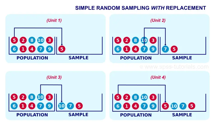
In real-world research, simple sampling with replacement is not common. This is because
respondents who are “sampled” a second or third time
will probably just tell the statistician to “f@#k off”.
Anyway. The syntax below demonstrates simple random sampling with replacement in SPSS. It uses both WEIGHT and FILTER in order for the sample to take effect.
Simple Random Sampling With Replacement Syntax
set seed 1.
do repeat #s = s1 to s50.
compute #s = rv.uni(0,1).
end repeat.
*2. Rank random numbers.
rank s1 to s50.
*3. Each rank variable represents a single draw with replacement.
recode rs1 to rs50 (2 thru hi = 0).
*4. The sum of our 50 draws is our sample variable.
compute sample = sum(rs1 to rs50).
*5. Inspect sample variable in data view.
sort cases by sample (d).
*6. Sample variable should sum to n = 50 cases.
descriptives sample/statistics min max mean sum.
*7. Filter not necessary but circumvents warning when WEIGHT is used.
filter by sample.
*8. Use sample as weight variable.
weight by sample.
*9. Descriptives on 50 cases.
descriptives id.
Result in Data View
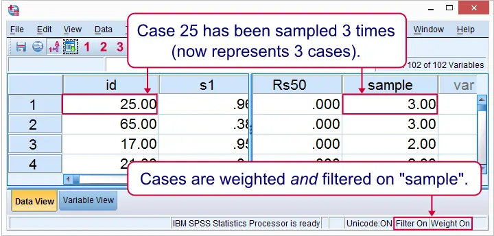
Right. So those are some basics on sampling in SPSS. I hope you found them helpful.
In any case, thanks for reading and keep up the good work!
Survey Sampling – Quick & Simple Introduction
When it's not feasible to study an entire target population, a simple random sample is the next best option; with sufficient sample size, it satisfies the assumption of independent and identically distributed variables. And perhaps even more important, it will tend to be nicely representative for the population with regard to all variables.
Although simple random sampling nicely satisfies two major statistical assumptions, we rarely see it in practice. This tutorial explains the reasons for this discrepancy. Before discussing the steps in a typical survey sampling procedure, we'll first give a quick overview of the process.
Survey Sampling - Quick Overview
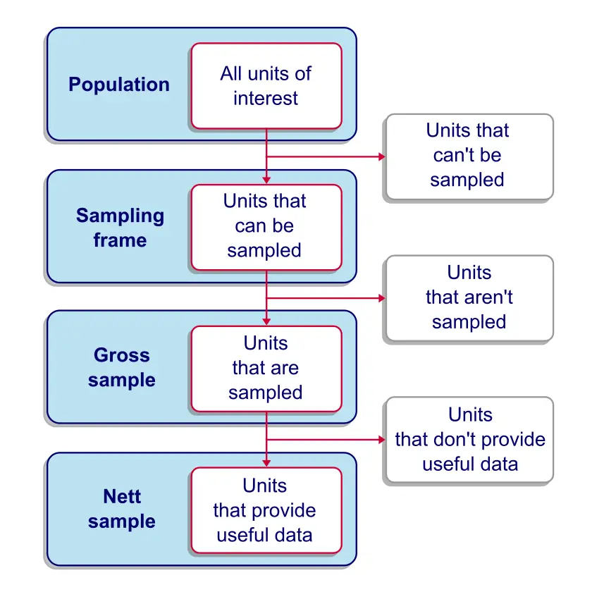
Survey Sampling - The Sampling Frame
The sampling frame is the collection of units
that are available for our sampling procedure.
So what do we mean by that? Well, in many cases a substantial part of our population simply cannot be sampled due to practical reasons. Regarding a target population of people, we rarely have accurate contact information from each single person. If we want to conduct an online survey, then people whose contact information is absent or incorrect have a zero chance of ending up in our sample. For this case, the sampling frame consists of the people in our population whose contact information is available and correct.
A sampling frame we encounter a lot in practice is an (online) panel; commercial research agencies often maintain a database of people who are willing to participate in surveys on a regular basis. When drawing a sample from such a panel, people who don't participate in the panel have a zero chance of ending up in our sample.
Survey Sampling - Coverage
Coverage is the percentage of a target population
that's covered in the sampling frame.
For example, the Dutch government has the correct home addresses of almost all Dutch citizens because people are enforced by law to provide this information. If we'd have access to this database, we could draw a random sample from it. In this case, the database would be our sampling frame with a coverage perhaps as high as 99%.
Now, sampling frames with such high coverages will tend to be relatively representative. Sure, the 1% we're missing may have (very) different characteristics than our entire population. However, any bias caused by their exclusion will be limited because they're so small in number.
The opposite reasoning may or may not hold. That is,
a sampling frame with a small coverage
may or may not be representative.
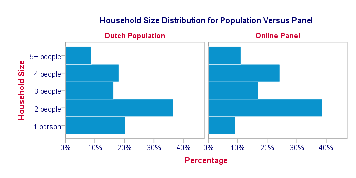
For instance, the main panel used by TNS NIPO contains some 213,000 respondents, roughly 1.36% of the Dutch population. However, this sampling frame with a mere 1.36% coverage is remarkably representative for the Dutch population (at least with regard to demographic variables). This is because the demographic makeup of this panel is constantly monitored and panel members are carefully selected from underrepresented groups. The illustration below gives an example.
A remark that's in place here is that a representative sampling frame is not always necessary for drawing a representative sample. In some cases, relevant (demographic) background variables are known for the sampling frame as well as the target population. If so, one can oversample underrepresented groups and undersample overrepresented groups, resulting in a representative gross sample. This procedure is very similar to weighting. But let's first take a look at the gross sample.
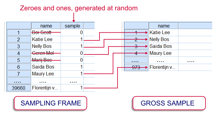
Survey Sampling - The Gross Sample
A gross sample is the collection of units that are sampled, regardless whether (usable) data is obtained from them.
With regard to surveying people, a gross sample is the group of people who are asked to participate in a survey. In some cases (especially online questionnaires) the gross sample may correspond to the sampling frame; we can simply send out our survey to everyone whose contact details we have.
However, some surveys still use face-to-face or phone interviews or paper questionnaires. In case of a huge sampling frame, approaching it entirely may be costly. This is one major reason for sampling from the sampling frame. In practice, the gross sample is often a simple random sample (without replacement) from the sampling frame. The illustration shows how it's typically done in SPSS.
Regarding online panel research, questionnaires are rarely sent out to the entire panel because we don't want to bother the panel members with too many questionnaires. On top of limiting such “respondent burden”, panel members often receive (monetary) incentives for answering questionnaires. This renders it costly to approach an entire (online) panel for a survey.
Survey Sampling - The Nett Sample
A nett sample is the collection of units
from which useful data are obtained.
Other than physical objects or animals, people often decline when we try to collect data on them. This phenomenon is aptly named non response. The percentage of a gross sample who do participate in a survey is known as the response rate.
For many studies, response rates typically hover around 20%. This can often be raised by offering incentives or sending out reminders. However, even panel members who clearly stated they're willing to participate in surveys rarely show response rates over some 70%.
After collecting data from the participants, it often turns out that some of them gave nonsensical answers or skipped many questions. We typically remove such respondents altogether from our data. The respondents who do provide us with useful data constitute the nett sample.
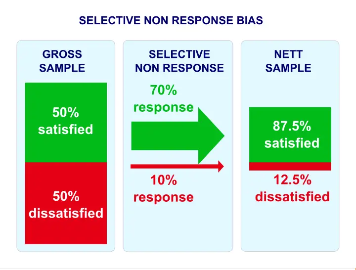
Survey Sampling - Selective Non Response
Selective non response is non response that's associated with one or more variables that are relevant for the study.
Example: we conduct a customer satisfaction study. In reality, 50% of our customers are satisfied and another 50% are dissatisfied. The same percentages are present in our gross sample. Now, our satisfied customers are willing to help out, resulting in a 70% response rate. Less happy customers may be unwilling to participate, resulting in a 10% response rate.
In other words: the response rate is associated with customer satisfaction -the single most relevant variable in the entire study. This selective non response results in a nett sample containing 85% satisfied customers. The situation is illustrated by the figure below.
Survey Sampling - Weighting
Weighting is having single observations “count as”
more or less than single observations.
For example, a (nett) sample consists of 30 females and 10 males. In this case, we may want to weight this sample: we'll have each female respondent count as only 0.67 respondents and each male respondent as 2 respondents. The figure below shows what this looks like in our data.
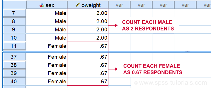 A weighted nett sample. Note that the weights are just a variable in our data.
Now 30 females will count as (30 * 0.67 =) 20 respondents and 10 men count as (10 * 2 =) 20 respondents. The weighted sample now consists of 20 males and 20 females.
What the previous example illustrated is that selective non response biases research outcomes. It does so by affecting the representativity of the nett sample.
So how can we prevent bias from selective non response?
The most common “fix” to selective non response is weighting the nett sample. A detailed explanation of weighting is beyond the scope of this tutorial.However, see SPSS WEIGHT Command Very briefly, weighting means that underrepresented groups are given more weight in the sample and vice versa for overrepresented groups. The result is a weighted nett sample that may be more representative than its unweighted counterpart.
Importantly, weighting requires that population distributions on relevant background variables are known (or can be reasonably estimated) for the target population. In practice, such frequency distributions are often available only for very general populations (such as all Dutch citizens) on main demographic variables (age, gender). Unfortunately, this information is often insufficient in order to properly weight a sample.
Finally, keep in mind here that weighting violates simple random sampling and therefore biases inferential statistics (such as p-values and confidence intervals) unless special corrections are used.