SPSS Two-Way ANOVA with Interaction Tutorial

Introduction & Practice Data File

Do you think running a two-way ANOVA with an interaction effect is challenging? Then this is the tutorial for you. We'll run the analysis by following a simple flowchart and we'll explain each step in simple language. After reading it, you'll know what to do and you'll understand why.
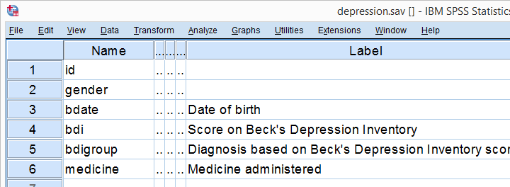
We'll use depression.sav throughout. The screenshot below shows it in variable view.

Research Questions

Very basically, 100 participants suffering from depression were divided into 4 groups of 25 each. Each group was given a different medicine. After 4 weeks, participants filled out the BDI, short for Beck's depression inventory. Our main research question is: did our different medicines result in different mean BDI scores? A secondary question is whether the BDI scores are related to gender in any way. In short we'll try to gain insight into 4 (medicines) x 2 (gender) = 8 mean BDI scores.

Quick Check: Histogram over Scores

Before jumping blindly into statistical tests, let's first see if our BDI scores make any sense in the first place. Before analyzing any metric variable, I always first inspect its histogram. The fastest way to create it is running the syntax below.

Result

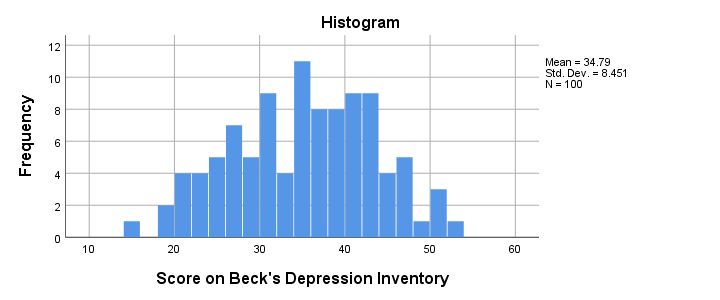
The scores look fine. We've perhaps one outlier who scores only 15 but we'll leave it in the data. The scores are roughly normally distributed and there's no need to specify any missing values.

ANOVA Assumptions

When we compare more than 2 means, we usually do so by ANOVA -short for analysis of variance. Doing so requires our data to meet the following assumptions:

• Independent observations (or independent and identically distributed variables). This often holds if each case contains a distinct person and the participants didn't interact.
• Homogeneity: the population variances are all equal over subpopulations. Violation of this assumption is less serious insofar as sample sizes are equal.
• Normality: the test variable must be normally distributed in each subpopulation. This assumption becomes less important insofar as the sample sizes are larger.

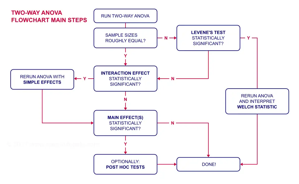
ANOVA Flowchart

Inspecting Means and Sample Sizes

The first question in our ANOVA flowchart is whether the sample sizes are roughly equal. I like to run a means table for inspecting this because I'm going to need this table anyway for my report. I'll create it with the syntax below.

Result

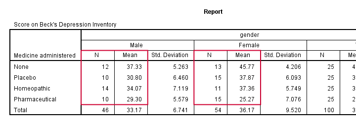
Note that this table shows the 8 means (2 genders * 4 medicines) that our analysis is all about. Each of these 8 means is based on 10 through 15 observations so the sample sizes are roughly equal.
This means that we don't need to bother about the homogeneity assumption. We can therefore skip Levene's test as shown in our flowchart.

Running Two-Way ANOVA in SPSS

We'll now run our two-way ANOVA through Analyze General Linear Model Univariate. We'll then follow the screenshots below.

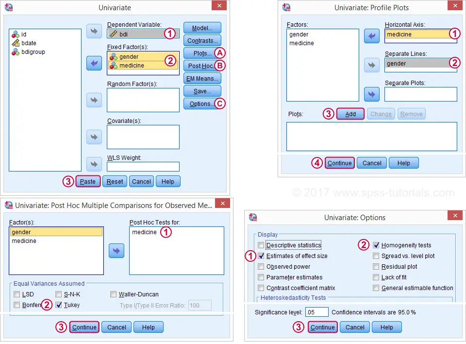
This results in the syntax below. Let's run it and see what happens.

ANOVA Output - Between Subjects Effects

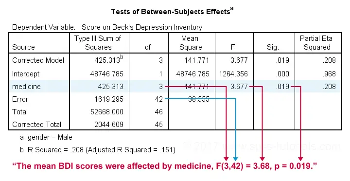
Following our flowchart, we should now find out if the interaction effect is statistically significant. A -somewhat arbitrary- convention is that an effect is statistically significant if “Sig.” < 0.05. According to the table below, our 2 main effects and our interaction are all statistically significant.

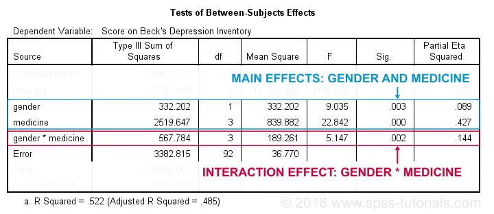
The flowchart says we should now rerun our ANOVA with simple effects. For now, we'll ignore the main effects -even if they're statistically significant. But why?! Well, this will become clear if we understand what our interaction effect really means. So let's inspect our profile plots.

ANOVA Output - Profile Plots

The profile plot shown below basically just shows the 8 means from our means table.If you ran the ANOVA like we just did, the “Estimated Marginal Means” are always the same as the observed means that we saw earlier. Interestingly, it also shows how medicine and gender affect these means.

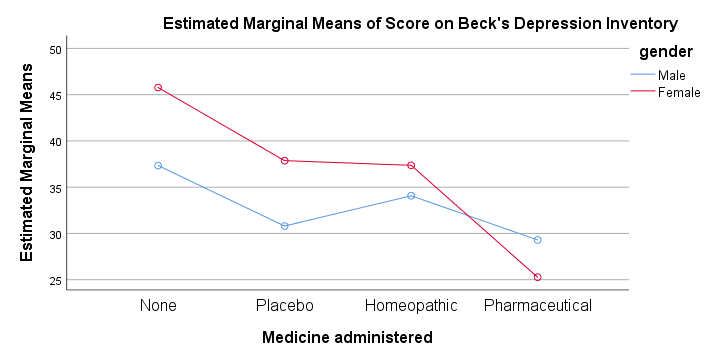
An interaction effect means that the effect of one factor depends on the other factor and it's shown by the lines in our profile plot not running parallel.
In this case, the effect for medicine interacts with gender. That is, medicine affects females differently than males. Roughly, we see the red line (females) descent quite steeply from “None” to “Pharmaceutical” whereas the blue line (males) is much more horizontal. Since it depends on gender, there's no such thing as the effect of medicine. So that's why we ignore the main effect of medicine -even if it's statistically significant. This main effect “lumps together” the different effects for males and females and this obscures -rather than clarifies- how medicine really affects the BDI scores.

Interaction Effect? Run Simple Effects.

So what should we do? Well, if medicine affects males and females differently, then we'll analyze male and female participants separately: we'll run a one-way ANOVA for just medicine on either group. This is what's meant by “simple effects” in our flowchart.

ANOVA with Simple Effects - Split File

How can we analyze 2 (or more) groups of cases separately? Well, SPSS has a terrific solution for this, known as SPLIT FILE. It requires that we first sort our cases so we'll do so as well.

Minor note: SPLIT FILE does not change your data in any way. It merely affects your output as we'll see in a minute. You can simply undo it by running SPLIT FILE OFF. but don't do so yet; we first want to run our one-way ANOVAs for inspecting our simple effects.

ANOVA with Simple Effects in SPSS

Since we switched on our SPLIT FILE, we can now just run one-way ANOVAs. We'll use Analyze General Linear Model Univariate. The screenshots below guide you through the next steps.

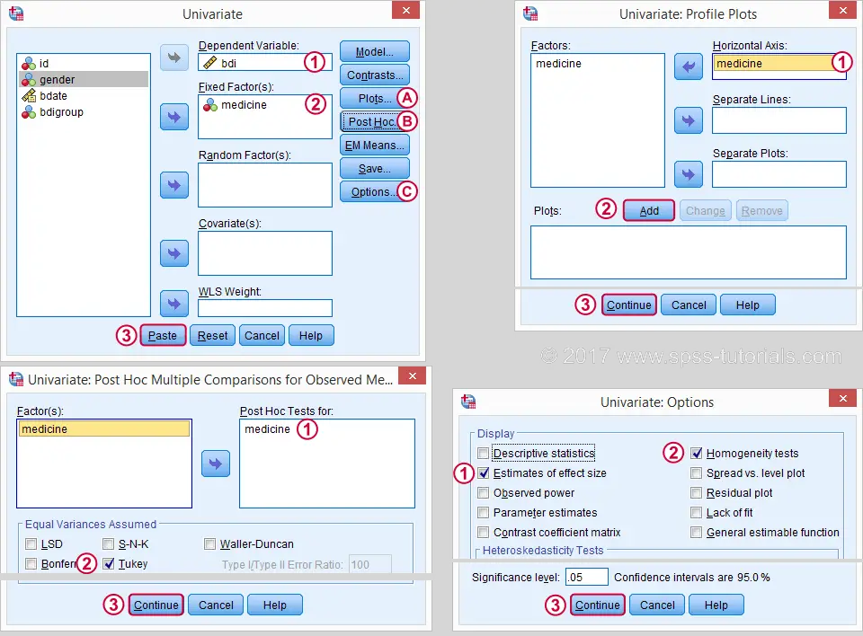
This results in the syntax below. Let's run it.

ANOVA Output - Between Subjects Effects

First off, note that the output window now contains all ANOVA results for male participants and then a similar set of results for females. According to our flowchart we should now inspect the main effect.

The effect for medicine is statistically significant. However, this just means it's probably not zero. But it's not very strong either as indicated by its partial eta squared of 0.208. This shouldn't come as a surprise. The 4 medicines don't differ much for males as we saw in our profile plots.

ANOVA Output - Post Hoc Tests

Our main effect suggests that our 4 medicines did not all perform similarly. But which one(s) really differ from which other one(s)? This question is addressed by our post hoc tests, in this case Tukey's HSD (“honestly significant differences”) comparisons.

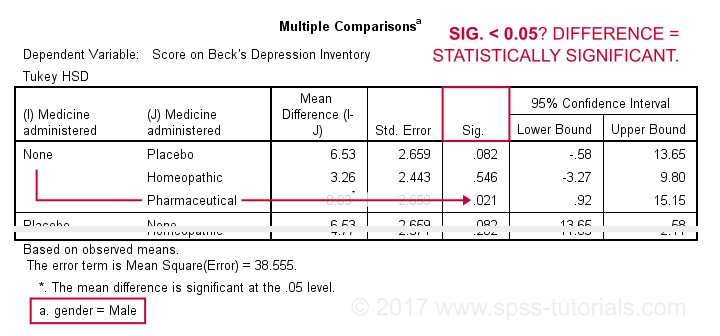
This table compares each medicine with each other medicine (twice). The only comparison yielding p < 0.05 is “None” versus “Pharmaceutical”. Our profile plots show that these are the worst and best performing medicines for male participants. The means for all other medicines are too close to differ statistically significantly.

Female Participants

According to our flowchart, we're now done -at least for males. Interpreting the results for female participants is left as an exercise for the reader. However, I do want to point out the following:

• our profile plots show a much steeper line for females than for males.
• the main effect of medicine has a much higher partial eta squared of 0.63 for females.
• the effect of medicine has p = 0.000 for females and p = 0.019 for males.
• for females, all post hoc comparisons are statistically significant except for “Homeopathic” versus “Placebo” (p = 0.997).

All these findings indicate a much stronger effect of medicine for females than for males; there's a substantial interaction effect between medicine and gender on BDI scores. And this -again- is the reason why we need to analyze these groups separately and rerun our ANOVA with simple effects -like we just did.

Final Notes

Do you still think running a two-way ANOVA with an interaction effect is challenging? I hope this tutorial helped you understand the main line of thinking. And -hopefully!- things start to sink in for you -perhaps after a second reading.

SPSS Two Way ANOVA – Basics Tutorial

Research Question

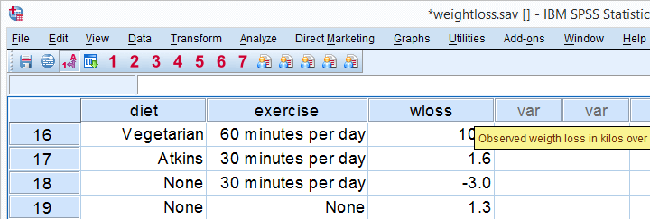
How to lose weight effectively? Do diets really work and what about exercise? In order to find out, 180 participants were assigned to one of 3 diets and one of 3 exercise levels. After two months, participants were asked how many kilos they had lost. These data -partly shown above- are in weightloss.sav.
We're going to test if the means for weight loss after two months are the same for diet, exercise level and each combination of a diet with an exercise level. That is, we'll compare more than two means so we end up with some kind of ANOVA.

Case Count and Histogram

We always want to have a basic idea what our data look like before jumping into any analyses. We first want to confirm that we really do have 180 cases. Next, we'd like to inspect the frequency distribution for weight loss with a histogram. We'll do so by running the syntax below.

Result

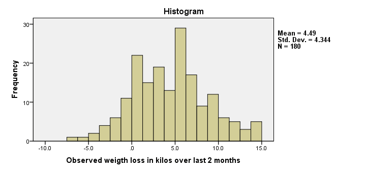
We have 180 cases indeed. Importantly, the histogram of weight loss looks plausible. We don't see any very high or low values that we should set as user missing values. One or two participants gained some 7 kilos (weight loss = -7) and some managed to lose up to 15 kilos. Furthermore, weight loss looks reasonably normally distributed.

Contingency Table Diet by Exercise

We now like to know how participants are distributed over diet and exercise. For our ANOVA, later on, we need to know if our design is balanced: are the percentages of participants in each diet equal over exercise levels? Some of you may notice that this question is actually the null hypothesis in a chi-square test. And that's exactly what we'll run next.

Result

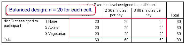
Note that each cell (combination of diet and exercise level) holds 20 participants. Note that our chi-square value is 0 (not shown in screenshot). This implies that we're dealing with a balanced design, which is a good thing because unbalanced designs somewhat complicate a two-way ANOVA.

Means Table

So did the diet and exercise have any effect? A very simple way for getting an idea of this is running a basic MEANS table.

Result

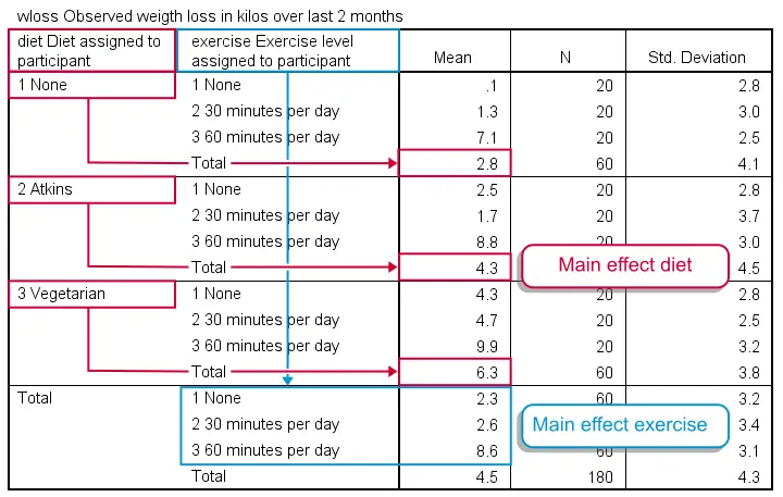
It may take a minute to see the pattern in this table but I did my best to highlight it with colors. Note that participants without any diet -all exercise levels taken together- lost an average of 2.8 kilos. The Atkins and vegetarian diets resulted in 6.3 and 4.3 kilos of weight loss on average. This is the main effect for diet: the differences in weight loss attributable to diet while taking together all exercise levels. In a similar vein, we see a somewhat stronger main effect for exercise with means running from 2.3 up to 8.6 kilos.
An interesting question is whether the effect of exercise depends on the diet followed. This is what we call an interaction effect. We'll explain it in a minute by visualizing our means in a chart.

Two Way ANOVA - Basic Idea

We just saw that different diets and exercise levels show different mean weight losses. However, we're looking at just a tiny sample. The situation in the (much larger) population may be different. Is it credible that we find these differences if neither diet nor exercise has any effect whatsoever in our population? We'll answer this question by running a two way ANOVA.

ANOVA Assumptions

In short, the main statistical assumptions required for ANOVA are

• independent observations: this often means that each case (row of data values) must represent a separate person (or other “object”). It's not allowed for a single person to appear as more than one case, which holds for our data.
• homoscedasticity: the standard deviation of our dependent variable (weight loss) must be equal for each (diet/exercise) group of respondents. Our previous means table shows that they are pretty similar indeed. Nevertheless, we'll also test this assumption more formally with Levene's test which is included in SPSS ANOVA procedure.
• a normally distributed dependent variable in the population. Our previous histogram suggests this holds for our data. On top of that, the normality assumption is of minor importance for larger sample sizes due to the central limit theorem.

SPSS Two Way ANOVA Menu

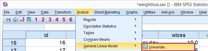
We choose Univariate whenever we analyze just one dependent variable (weight loss), regardless how many independent variables (diet and exercise) we may have.

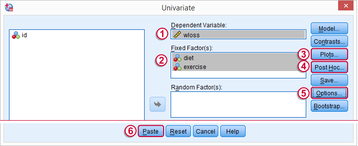
Before pasting the syntax, we'll quickly jump into the subdialogs , and for adjusting some settings.

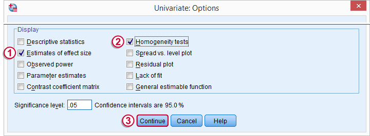
Estimates of effect size will add partial eta squared in our output.
Homogeneity tests refers to Levene’s test. It assesses whether the population variances of our dependent variable are equal over the levels of our factors. This assumption is required for ANOVA.

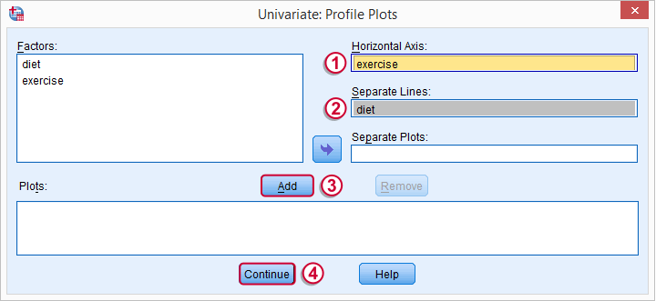
Profile plots visualize means for each combination of factors. As we'll see in a minute, this gives a lot of insight into how our factors relate to our dependent variable and -possibly- interact while doing so.

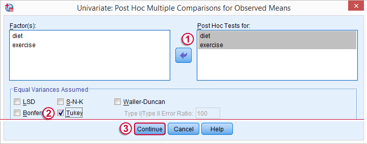
A basic ANOVA only tests the null hypothesis that all means are equal. If this is unlikely, then we'll usually want to know exactly which means are not equal. The most common post hoc test for finding out is Tukey’s HSD (short for Honestly Significant Difference).

SPSS Two Way ANOVA Syntax

Following through all steps results in the syntax below. We'll run it and discuss the results.

Two Way ANOVA Output - Levene’s Test

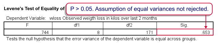
Levene’s test does not reject the assumption of equal variances that's needed for our ANOVA results later on. We're good to go. Let's scroll down to the end of our output now for our profile plots first.

Two Way ANOVA Output - Profile Plots

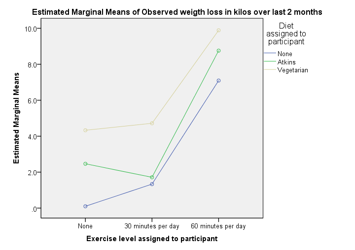
This basically says it all. We see each line rise steeply between 30 to 60 minutes of exercise per day. Second, a vegetarian diet always resulted in more weight loss than the other diets. Both diet and exercise seem to have a main effect on weight loss.
So what about our interaction effect? Well, the effect of exercise is visualized as a line for each diet group separately. Since these lines look pretty similar, our plot doesn't show much of an interaction effect. However, we'll try to confirm this with a more formal test in a minute.
Technical note: the “estimated marginal means” are equal to the observed means in our previous means table because we tested the saturated model (consisting of all main and interaction effects as this is the default setting in UNIANOVA).

Two Way ANOVA Output - Between Subjects Effects

Our means plot was very useful for describing the pattern of means resulting from diet and exercise in our sample. But perhaps things are different in the larger population. If neither diet nor exercise affect weight loss, could we find these sample results by mere sampling fluctuation? Short answer: no.

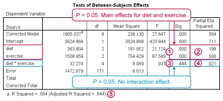
In Tests of Between-Subjects Effects, we're interested in 3 rows: our 2 main effects (diet and exercise) and 1 interaction effect (diet * exercise). We usually ignore the other rows such as “Corrected Model” and “Intercept”.
First the interaction: if the effect of exercise is the same for all diets, then there's a 0.44 probability (p-value under “Sig” for “significance”) of finding our sample results. We usually report our df (“degrees of freedom”), F-value and p-value for each of our 3 effects separately: “An interaction between diet and exercise could not be demonstrated, F(4,171) = .94, p = 0.44.” Further note that partial eta squared is only 0.021 for our interaction effect. This is basically negligible.
If and only if there's no interaction effect, we'll look into the main effects, both of which have p = 0.000: if there's no main effects in our larger population, the probability of finding these sample main effects is basically zero.
Partial eta squared is 0.51 for exercise and 0.20 for diet. That is, the relative impact of exerice is more than twice as strong as diet.
Last but not least, adjusted r squared tells us that 54.4% of the variance in weight loss is attributable to diet and exercise. In social sciences research, this is a high value, indicating strong relationships between our factors and weight loss.

Two Way ANOVA Output - Multiple Comparisons

We now know that the average weight loss is not equal for all different diets and exercise levels. So precisely which means are different? We can figure that out with post hoc tests, the most common of which is Tukey’s HSD, the output of which is shown below.

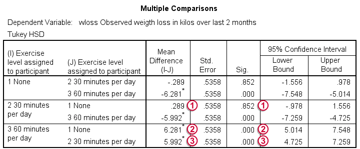
For 3 means, 3 comparisons are made (a-b, b-c and a-c). Each is reported twice in this table, resulting in 6 rows.
The difference in weight loss between no exercise and 30 minutes is 0.29 kilos. If it is zero in our larger populations, there's an 85.2% probability of finding this in our sample. Our results don't demonstrate any effect of 30 minutes of exercise as compared to no exercise.
The difference between no exercise and 60 minutes is a whopping 6.28 kilos. Both the asterisk (*), confidence interval and p-value show that the difference is statistically significant.
A similar table for diet appears in the output but we'll leave it as an exercise to the reader to interpret it.

So that's about it. I hope you were able to follow the lines of thought in this tutorial and that they make some sense to you.