SPSS - Kendall’s Concordance Coefficient W

SPSS – Kendall’s Concordance Coefficient W

Kendall’s Concordance Coefficient W is a number between 0 and 1
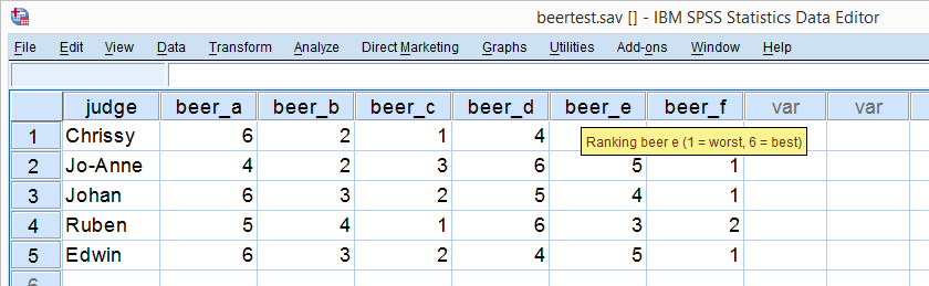
that indicates interrater agreement. So let's say we had 5 people rank 6 different beers as shown below. We obviously want to know which beer is best, right? But could we also quantify how much these raters agree with each other? Kendall’s W does just that.

Kendall’s W - Example

So let's take a really good look at our beer test results. The data -shown above- are in beertest.sav. For answering which beer was rated best, a Friedman test would be appropriate because our rankings are ordinal variables. A second question, however, is to what extent do all 5 judges agree on their beer rankings? If our judges don't agree at all which beers were best, then we can't possibly take their conclusions very seriously. Now, we could say that “our judges agreed to a large extent” but we'd like to be more precise and express the level of agreement in a single number. This number is known as Kendall’s Coefficient of Concordance W.^2,3

Kendall’s W - Basic Idea

Let's consider the 2 hypothetical situations depicted below: perfect agreement and perfect disagreement among our raters. I invite you to stare at it and think for a minute.

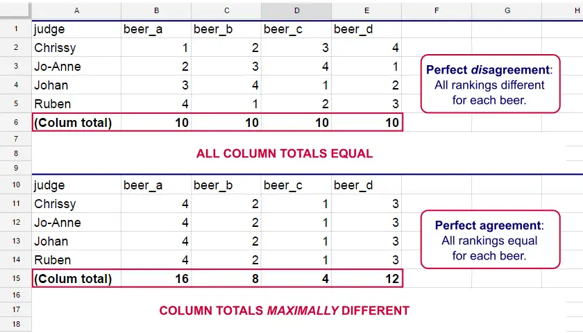
Kendalls Concordance Coefficient - Basic Idea

As we see, the extent to which raters agree is indicated by the extent to which the column totals differ. We can express the extent to which numbers differ as a number: the variance or standard deviation.
Kendall’s W is defined as

$$W = \frac{Variance\,over\,column\,totals}{Maximum\,possible\,variance\,over\,column\,totals}$$

As a result, Kendall’s W is always between 0 and 1. For instance, our perfect disagreement example has W = 0; because all column totals are equal, their variance is zero.
Our perfect agreement example has W = 1 because the variance among column totals is equal to the maximal possible variance. No matter how you rearrange the rankings, you can't possibly increase this variance any further. Don't believe me? Give it a go then.
So what about our actual beer data? We'll quickly find out with SPSS.

Kendall’s W in SPSS

We'll get Kendall’s W from SPSS’ Nonparametric Tests menu. The screenshots below walk you through.

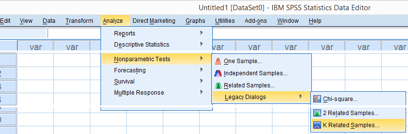
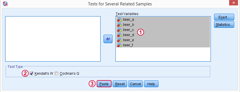
SPSS Kendalls Concordance Coefficient - Main Menu

Note: SPSS thinks our rankings are nominal variables. This is because they contain few distinct values. Fortunately, this won't interfere with the current analysis. Completing these steps results in the syntax below.

Kendall’s W - Basic Syntax

*Kendall's W from nonparametric tests - legacy dialogs - k related samples.

NPAR TESTS
/KENDALL=beer_a beer_b beer_c beer_d beer_e beer_f
/MISSING LISTWISE.

Kendall’s W - Output

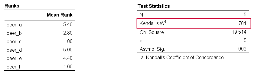
And there we have it: Kendall’s W = 0.78. Our beer judges agree with each other to a reasonable but not super high extent. Note that we also get a table with the (column) mean ranks that tells us which beer was rated most favorably.

Average Spearman Correlation over Judges

Another measure of concordance is the average over all possible Spearman correlations among all judges.¹ It can be calculated from Kendall’s W with the following formula

$$\overline{R}_s = {kW - 1 \over k - 1}$$

where $\overline{R}_s$ denotes the average Spearman correlation and $k$ the number of judges. For our example, this comes down to

$$\overline{R}_s = {5(0.781) - 1 \over 5 - 1} = 0.726$$

We'll verify this by running and averaging all possible Spearman correlations in SPSS. We'll leave that for a next tutorial, however, as doing so properly requires some highly unusual -but interesting- syntax.

Thank you for reading!

References

Howell, D.C. (2002). Statistical Methods for Psychology (5th ed.). Pacific Grove CA: Duxbury.
Slotboom, A. (1987). Statistiek in woorden [Statistics in words]. Groningen: Wolters-Noordhoff.
Van den Brink, W.P. & Koele, P. (2002). Statistiek, deel 3 [Statistics, part 3]. Amsterdam: Boom.

Cramér’s V – What and Why?

Cramér’s V is a number between 0 and 1 that indicates how strongly two categorical variables are associated. If we'd like to know if 2 categorical variables are associated, our first option is the chi-square independence test. A p-value close to zero means that our variables are very unlikely to be completely unassociated in some population. However, this does not mean the variables are strongly associated; a weak association in a large sample size may also result in p = 0.000.

Cramér’s V - Formula

A measure that does indicate the strength of the association is Cramér’s V, defined as

$$\phi_c = \sqrt{\frac{\chi^2}{N(k - 1)}}$$

where

$\phi_c$ denotes Cramér’s V;$\phi$ is the Greek letter “phi” and refers to the “phi coefficient”, a special case of Cramér’s V which we'll discuss later.
$\chi^2$ is the Pearson chi-square statistic from the aforementioned test;
$N$ is the sample size involved in the test and
$k$ is the lesser number of categories of either variable.

Cramér’s V - Examples

A scientist wants to know if music preference is related to study major. He asks 200 students, resulting in the contingency table shown below.

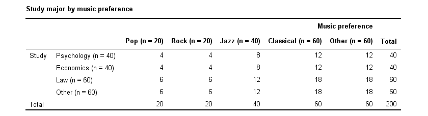
These raw frequencies are just what we need for all sort of computations but they don't show much of a pattern. The association -if any- between the variables is easier to see if we inspect row percentages instead of raw frequencies. Things become even clearer if we visualize our percentages in stacked bar charts.

Cramér’s V - Independence

In our first example, the variables are perfectly independent: $\chi^2$ = 0. According to our formula, chi-square = 0 implies that Cramér’s V = 0. This means that music preference “does not say anything” about study major. The associated table and chart make this clear.

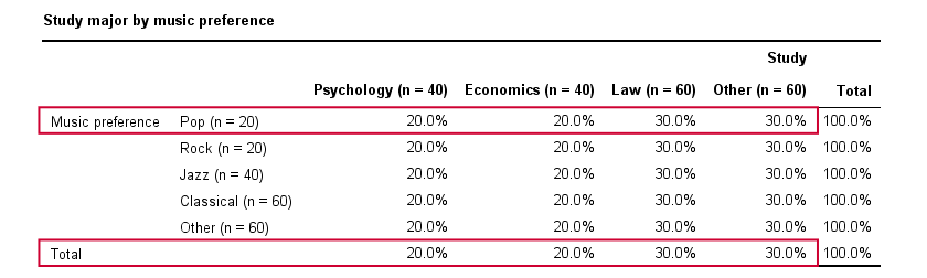
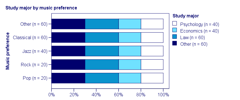
Cramers V Crosstab Unassociated Percentages

Note that the frequency distribution of study major is identical in each music preference group. If we'd like to predict somebody’s study major, knowing his music preference does not help us the least little bit. Our best guess is always law or “other”.

Cramér’s V - Moderate Association

A second sample of 200 students show a different pattern. The row percentages are shown below.

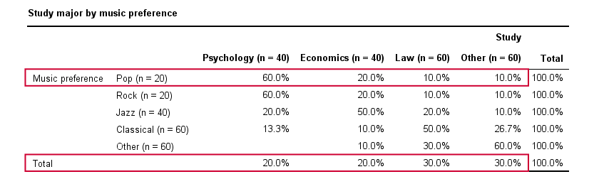
This table shows quite some association between music preference and study major: the frequency distributions of studies are different for music preference groups. For instance, 60% of all students who prefer pop music study psychology. Those who prefer classical music mostly study law. The chart below visualizes our table.

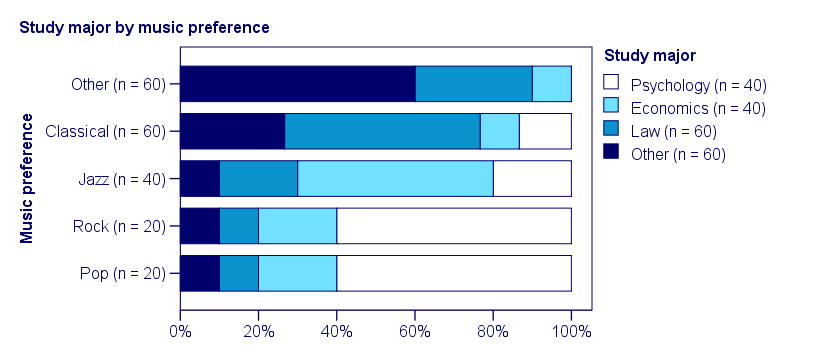
Note that music preference says quite a bit about study major: knowing the former helps a lot in predicting the latter. For these data

$\chi^2 \approx$ 113;For calculating this chi-square value, see either Chi-Square Independence Test - Quick Introduction or SPSS Chi-Square Independence Test.
our sample size N = 200 and
we've variables with 4 and 5 categories so k = (4 -1) = 3.

It follows that

$$\phi_c = \sqrt{\frac{113}{200(3)}} = 0.43.$$

which is substantial but not super high since Cramér’s V has a maximum value of 1.

Cramér’s V - Perfect Association

In a third -and last- sample of students, music preference and study major are perfectly associated. The table and chart below show the row percentages.

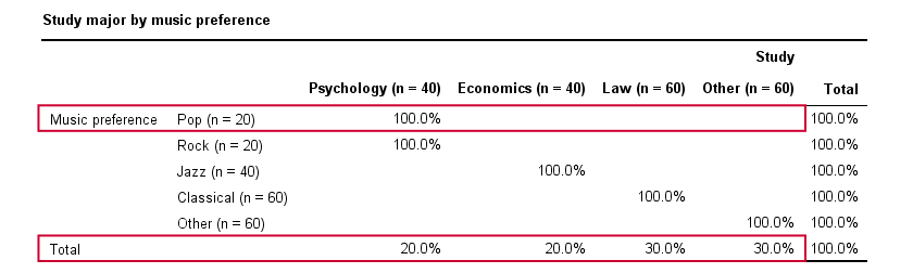
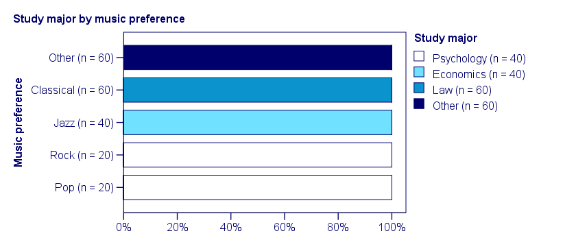
If we know a student’s music preference, we know his study major with certainty. This implies that our variables are perfectly associated. Do notice, however, that it doesn't work the other way around: we can't tell with certainty someone’s music preference from his study major but this is not necessary for perfect association: $\chi^2$ = 600 so

$$\phi_c = \sqrt{\frac{600}{200(3)}} = 1,$$

which is the very highest possible value for Cramér’s V.

Alternative Measures

An alternative association measure for two nominal variables is the contingency coefficient. However, it's better avoided since its maximum value depends on the dimensions of the contingency table involved.^3,4
For two ordinal variables, a Spearman correlation or Kendall’s tau are preferable over Cramér’s V.
For two metric variables, a Pearson correlation is the preferred measure.
If both variables are dichotomous (resulting in a 2 by 2 table) use a phi coefficient, which is simply a Pearson correlation computed on dichotomous variables.

Cramér’s V - SPSS

In SPSS, Cramér’s V is available from Analyze Descriptive Statistics Crosstabs. Next, fill out the dialog as shown below.

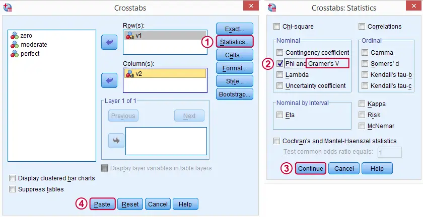
Warning: for tables larger than 2 by 2, SPSS returns nonsensical values for phi without throwing any warning or error. These are often > 1, which isn't even possible for Pearson correlations. Oddly, you can't request Cramér’s V without getting these crazy phi values.

Final Notes

Cramér’s V is also known as Cramér’s phi (coefficient)⁵. It is an extension of the aforementioned phi coefficient for tables larger than 2 by 2, hence its notation as $\phi_c$. It's been suggested that its been replaced by “V” because old computers couldn't print the letter $\phi$.³

Thank you for reading.

References

Van den Brink, W.P. & Koele, P. (2002). Statistiek, deel 3 [Statistics, part 3]. Amsterdam: Boom.
Field, A. (2013). Discovering Statistics with IBM SPSS Newbury Park, CA: Sage.
Howell, D.C. (2002). Statistical Methods for Psychology (5th ed.). Pacific Grove CA: Duxbury.
Slotboom, A. (1987). Statistiek in woorden [Statistics in words]. Groningen: Wolters-Noordhoff.
Sheskin, D. (2011). Handbook of Parametric and Nonparametric Statistical Procedures. Boca Raton, FL: Chapman & Hall/CRC.