SPSS Moderation Regression Tutorial
- SPSS Moderation Regression - Example Data
- SPSS Moderation Regression - Dialogs
- SPSS Moderation Regression - Coefficients Output
- Simple Slopes Analysis I - Fit Lines
- Simple Slopes Analysis II - Coefficients
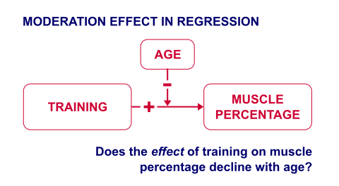
A sports doctor routinely measures the muscle percentages of his clients. He also asks them how many hours per week they typically spend on training. Our doctor suspects that clients who train more are also more muscled. Furthermore, he thinks that the effect of training on muscularity declines with age. In multiple regression analysis, this is known as a moderation interaction effect. The figure below illustrates it.
So how to test for such a moderation effect? Well, we usually do so in 3 steps:
- if both predictors are quantitative, we usually mean center them first;
- we then multiply the centered predictors into an interaction predictor variable;
- finally, we enter both mean centered predictors and the interaction predictor into a regression analysis.
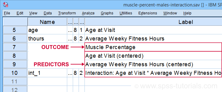
SPSS Moderation Regression - Example Data
These 3 predictors are all present in muscle-percent-males-interaction.sav, part of which is shown below.
We did the mean centering with a simple tool which is downloadable from SPSS Mean Centering and Interaction Tool.
Alternatively, mean centering manually is not too hard either and covered in How to Mean Center Predictors in SPSS?
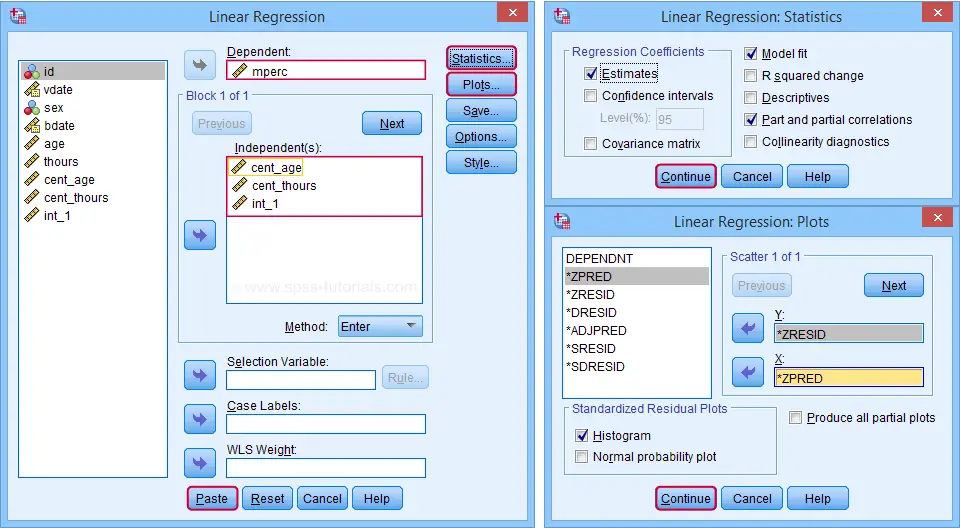
SPSS Moderation Regression - Dialogs
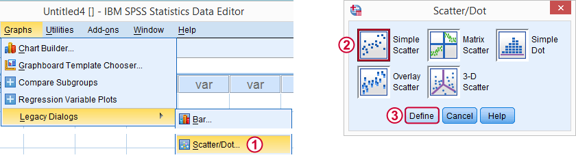
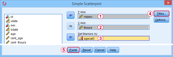
Our moderation regression is not different from any other multiple linear regression analysis: we navigate to
![]()
![]() and fill out the dialogs as shown below.
and fill out the dialogs as shown below.
Clicking results in the following syntax. Let's run it.
REGRESSION
/MISSING LISTWISE
/STATISTICS COEFF OUTS R ANOVA ZPP
/CRITERIA=PIN(.05) POUT(.10)
/NOORIGIN
/DEPENDENT mperc
/METHOD=ENTER cent_age cent_thours int_1
/SCATTERPLOT=(*ZRESID ,*ZPRED)
/RESIDUALS HISTOGRAM(ZRESID).
SPSS Moderation Regression - Coefficients Output
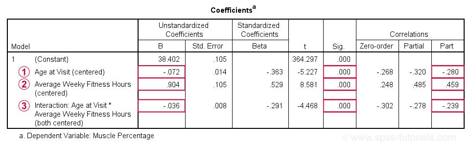
 Age is negatively related to muscle percentage. On average, clients lose 0.072 percentage points per year.
 Training hours are positively related to muscle percentage: clients tend to gain 0.9 percentage points for each hour they work out per week.
 The negative B-coefficient for the interaction predictor indicates that the training effect becomes more negative -or less positive- with increasing ages.
Now, for any effect to bear any importance, it must be statistically significant and have a reasonable effect size.
At p = 0.000, all 3 effects are highly statistically significant. As effect size measures we could use the semipartial correlations (denoted as “Part”) where
- r = 0.10 indicates a small effect;
- r = 0.30 indicates a medium effect;
- r = 0.50 indicates a large effect.
The training effect is almost large and the age and age by training interaction are almost medium. Regardless of statistical significance, I think the interaction may be ignored if its part correlation r < 0.10 or so but that's clearly not the case here. We'll therefore examine the interaction in-depth by means of a simple slopes analysis.
With regard to the residual plots (not shown here), note that
- the residual histogram doesn't look entirely normally distributed but -rather- bimodal. This somewhat depends on its bin width and doesn't look too alarming;
- the residual scatterplot doesn't show any signs of heteroscedasticity or curvilinearity. Altogether, these plots don't show clear violations of the regression assumptions.
Creating Age Groups
Our simple slopes analysis starts with creating age groups. I'll go for tertile groups: the youngest, intermediate and oldest 33.3% of the clients will make up my groups. This is an arbitrary choice: we may just as well create 2, 3, 4 or whatever number of groups. Equal group sizes are not mandatory either and perhaps even somewhat unusual. In any case, the syntax below creates the age tertile groups as a new variable in our data.
rank age
/ntiles(3) into agecat3.
*Label new variable and values.
variable labels agecat3 'Age Tertile Group'.
value labels agecat3 1 'Youngest Ages' 2 'Intermediary Ages' 3 'Highest Ages'.
*Check descriptive statistics age per age group.
means age by agecat3
/cells count min max mean stddev.
Result
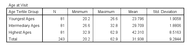
Some basic conclusions from this table are that
- our age groups have precisely equal sample sizes of n = 81;
- the group mean ages are unevenly distributed: the difference between young and intermediary -some 6 years- is much smaller than between intermediary and highest -some 13 years;
- the highest age group has a much larger standard deviation than the other 2 groups.
Points 2 and 3 are caused by the skewness in age and argue against using tertile groups. However, I think that having equal group sizes easily outweighs both disadvantages.
Simple Slopes Analysis I - Fit Lines
Let's now visualize the moderation interaction between age and training. We'll start off creating a scatterplot as shown below.
Clicking results in the syntax below.
GRAPH
/SCATTERPLOT(BIVAR)=thours WITH mperc BY agecat3
/MISSING=LISTWISE
/TITLE='Muscle Percentage by Training Hours by Age Group'.
*After running chart, add separate fit lines manually.
Adding Separate Fit Lines to Scatterplot
After creating our scatterplot, we'll edit it by double-clicking it. In the Chart Editor window that opens, we click the icon labeled Add Fit Line at Subgroups
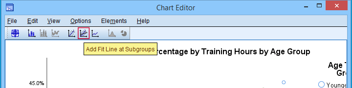
After adding the fit lines, we'll simply close the chart editor. Minor note: scatterplots with (separate) fit lines can be created in one go from the Chart Builder in SPSS version 25+ but we'll cover that some other time.
Result
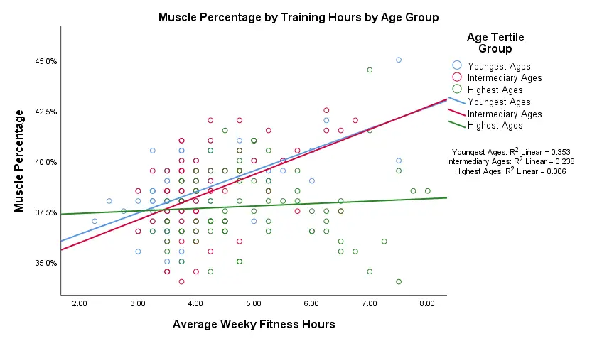
Our fit lines nicely explain the nature of our age by training interaction effect:
- the 2 youngest age groups show a steady increase in muscle percentage by training hours;
- for the oldest clients, however, training seems to hardly affect muscle percentage. This is how the effect of training on muscle percentage is moderated by age;
- on average, the 3 lines increase. This is the main effect of training;
- overall, the fit line for the oldest group is lower than for the other 2 groups. This is our main effect of age.
Again, the similarity between the 2 youngest groups may be due to the skewness in ages: the mean ages for these groups aren't too different but very different from the highest age group.
Simple Slopes Analysis II - Coefficients
After visualizing our interaction effect, let's now test it: we'll run a simple linear regression of training on muscle percentage for our 3 age groups separately. A nice way for doing so in SPSS is by using SPLIT FILE.
The REGRESSION syntax was created from the menu as previously but with (uncentered) training as the only predictor.
sort cases by agecat3.
split file layered by agecat3.
*Run simple linear regression with uncentered training hours on muscle percentage.
REGRESSION
/MISSING LISTWISE
/STATISTICS COEFF OUTS R ANOVA ZPP
/CRITERIA=PIN(.05) POUT(.10)
/NOORIGIN
/DEPENDENT mperc
/METHOD=ENTER thours
/SCATTERPLOT=(*ZRESID ,*ZPRED)
/RESIDUALS HISTOGRAM(ZRESID).
*Split file off.
split file off.
Result
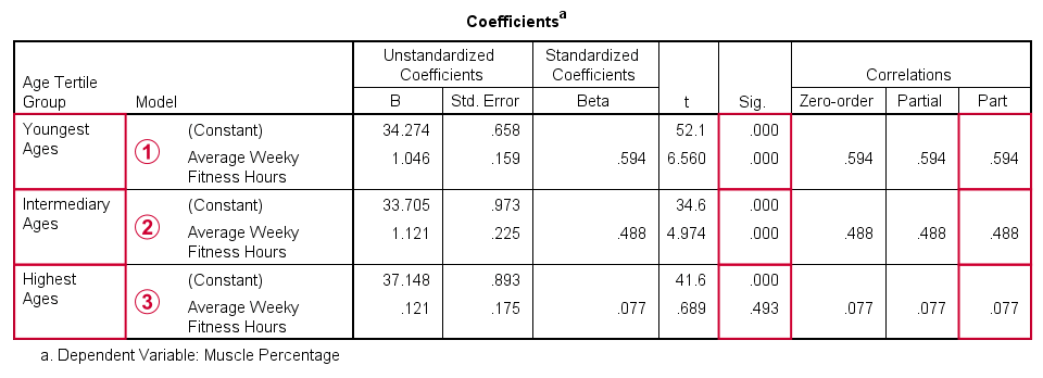
The coefficients table confirms our previous results:
for the youngest age group, the training effect is statistically significant at p = 0.000. Moreover, its part correlation of r = 0.59 indicates a large effect;
the results for the intermediary age group are roughly similar to the youngest group;
for the highest age group, the part correlation of r = 0.077 is not substantial. We wouldn't take it seriously even if it had been statistically significant -which it isn't at p = 0.49.
Last, the residual histograms (not shown here) don't show anything unusual. The residual scatterplot for the oldest age group looks curvilinear except from some outliers. We should perhaps take a closer look at this analysis but we'll leave that for another day.
Thanks for reading!
How to Mean Center Predictors in SPSS?
Also see SPSS Moderation Regression Tutorial.
For testing moderation effects in multiple regression, we start off with mean centering our predictors:
mean centering a variable is subtracting its mean
from each individual score.
After doing so, a variable will have a mean of exactly zero but is not affected otherwise: its standard deviation, skewness, distributional shape and everything else all stays the same.
After mean centering our predictors, we just multiply them for adding interaction predictors to our data. Mean centering before doing this has 2 benefits:
- it tends to diminish multicollinearity, especially between the interaction effect and its constituent main effects;
- it may render our b-coefficients more easily interpretable.
We'll cover an entire regression analysis with a moderation interaction in a subsequent tutorial. For now, we'll focus on
how to mean center predictors
and compute (moderation) interaction predictors?
Mean Centering Example I - One Variable
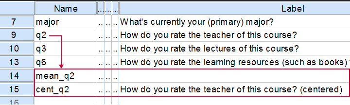
We'll now mean center some variables in course_evaluation.sav. Part of its variable view is shown below.
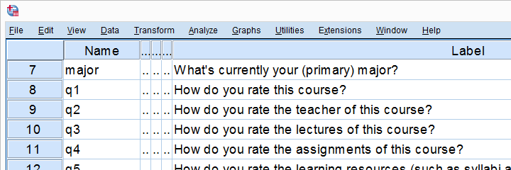
Let's start off with q2 (“How do you rate the teacher of this course?”). We'll first add this variable's mean as a new variable to our dataset with AGGREGATE.
The syntax below does just that. Don't bother about any menu here as it'll only slow you down.
Syntax for Adding a Variable's Mean to our Data
aggregate outfile * mode addvariables
/mean_q2 = mean(q2).
Result
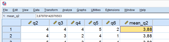
The mean for q2 seems to be 3.88.Sorry for the comma as a decimal separator here. I had my LOCALE set to Dutch when running this example. But oftentimes in SPSS,
what you see is not what you get.
If we select a cell, we see that the exact mean is 3.87978142076503. This is one reason why we don't just subtract 3.88 from our original variable -as proposed by many lesser tutorials.
A second reason is that our approach will still work perfectly if we decide to precede it with FILTER, SELECT IF or WEIGHT.
Right, now the second -and final- step is simply subtracting this mean from our original variable with COMPUTE. We'll then run a quick check on the result and we're done.
Subtracting the Mean from the Original Values
compute cent_q2 = q2 - mean_q2.
*Add variable label to centered variable.
variable labels cent_q2 "How do you rate the teacher of this course? (centered)".
*Check results.
descriptives q2 cent_q2.
*Delete helper variable.
delete variables mean_q2.
Result
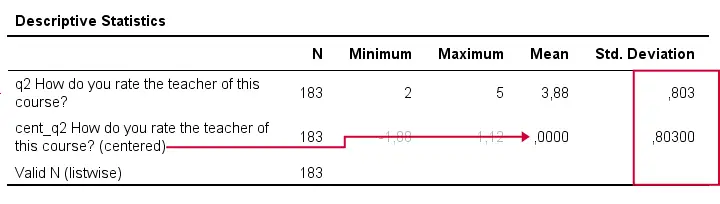
A quick check after mean centering is comparing some descriptive statistics for the original and centered variables:
- the centered variable must have an exactly zero mean;
- the centered and original variables must have the exact same standard deviations.
If these 2 checks hold, we can be pretty confident our mean centering was done properly.
Mean Centering Example II - Several Variables
In a real-life analysis, you'll probably center at least 2 variables because that's the minimum for creating a moderation predictor. You could mean center several variables by repeating the previous steps for each one.
However, it can be done much faster if we speed things up by
- throwing several variables into a single AGGREGATE command,
- using DO REPEAT for subtracting each variable's mean from the original scores and
- not creating helper variables holding means.
The syntax below does just that.
Syntax Example - Mean Center Several Variables
aggregate outfile * mode addvariables
/cent_q3 to cent_q6 = mean(q3 to q6).
*Subtract means from original variables.
do repeat #ori = q3 to q6 / #cent = cent_q3 to cent_q6.
compute #cent = #ori - #cent.
end repeat.
*Add variable labels to centered variables.
variable labels cent_q3 "How do you rate the lectures of this course? (centered)".
variable labels cent_q4 "How do you rate the assignments of this course? (centered)".
variable labels cent_q5 "How do you rate the learning resources (such as syllabi and handouts) that were issued by us? (centered)".
variable labels cent_q6 "How do you rate the learning resources (such as books) that were not issued by us? (centered)".
*Check results.
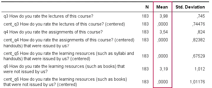
descriptives q3 cent_q3 q4 cent_q4 q5 cent_q5 q6 cent_q6.
Result
Adding Moderation Predictors to our Data
Although beyond the scope of this tutorial, creating moderation predictors is as simple as multiplying 2 mean centered predictors.
compute int_1 = cent_q3 * cent_q4.
*Apply short but clear variable label to interaction predictor.
variable labels int_1 "Interaction: lecture rating * assignment rating (both centered)".
For testing if q3 moderates the effect of q4 on some outcome variable, we simply enter this interaction predictor and its 2 mean centered(!) constituents, cent_q3, cent_q4 into our regression equation.
We'll soon cover the entire analysis (on more suitable data) in a subsequent tutorial.
Thanks for reading!