- Overview Transformations
- Normalizing - What and Why?
- Normalizing Negative/Zero Values
- Test Data
- Descriptives after Transformations
- Conclusion
Overview Transformations
| TRANSFORMATION | USE IF | LIMITATIONS | SPSS EXAMPLES |
|---|---|---|---|
| Square/Cube Root | Variable shows positive skewness Residuals show positive heteroscedasticity Variable contains frequency counts | Square root only applies to positive values | compute newvar = sqrt(oldvar). compute newvar = oldvar**(1/3). |
| Logarithmic | Distribution is positively skewed | Ln and log10 only apply to positive values | compute newvar = ln(oldvar). compute newvar = lg10(oldvar). |
| Power | Distribution is negatively skewed | (None) | compute newvar = oldvar**3. |
| Inverse | Variable has platykurtic distribution | Can't handle zeroes | compute newvar = 1 / oldvar. |
| Hyperbolic Arcsine | Distribution is positively skewed | (None) | compute newvar = ln(oldvar + sqrt(oldvar**2 + 1)). |
| Arcsine | Variable contains proportions | Can't handle absolute values > 1 | compute newvar = arsin(oldvar). |
Normalizing - What and Why?
“Normalizing” means transforming a variable in order to
make it more normally distributed.
Many statistical procedures require a normality assumption: variables must be normally distributed in some population. Some options for evaluating if this holds are
- inspecting histograms;
- inspecting if skewness and (excess) kurtosis are close to zero;
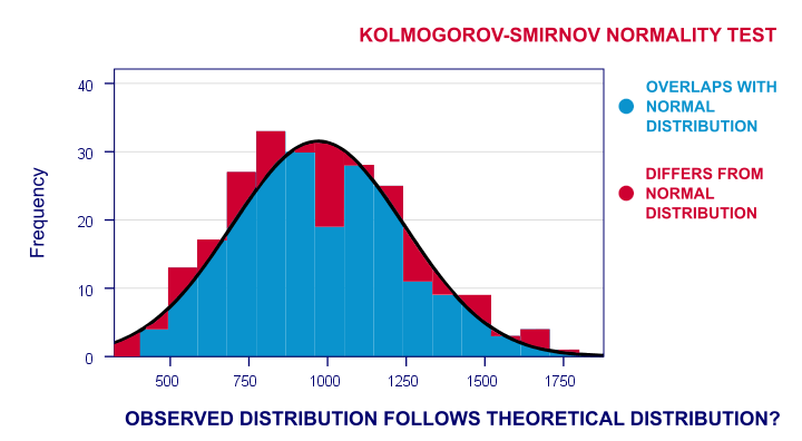
- running a Shapiro-Wilk test and/or a Kolmogorov-Smirnov test.
For reasonable sample sizes (say, N ≥ 25), violating the normality assumption is often no problem: due to the central limit theorem, many statistical tests still produce accurate results in this case. So why would you normalize any variables in the first place? First off, some statistics -notably means, standard deviations and correlations- have been argued to be technically correct but still somewhat misleading for highly non-normal variables.
Second, we also encounter normalizing transformations in multiple regression analysis for
- meeting the assumption of normally distributed regression residuals;
- reducing heteroscedasticity and;
- reducing curvilinearity between the dependent variable and one or many predictors.
Normalizing Negative/Zero Values
Some transformations in our overview don't apply to negative and/or zero values. If such values are present in your data, you've 2 main options:
- transform only non-negative and/or non-zero values;
- add a constant to all values such that their minimum is 0, 1 or some other positive value.
The first option may result in many missing data points and may thus seriously bias your results. Alternatively, adding a constant that adjusts a variable's minimum to 1 is done with
$$Pos_x = Var_x - Min_x + 1$$
This may look like a nice solution but keep in mind that a minimum of 1 is completely arbitrary: you could just as well choose, 0.1, 10, 25 or any other positive number. And that's a real problem because the constant you choose may affect the shape of a variable's distribution after some normalizing transformation. This inevitably induces some arbitrariness into the normalized variables that you'll eventually analyze and report.
Test Data
We tried out all transformations in our overview on 2 variables with N = 1,000:
- var01 has strong negative skewness and runs from -1,000 to +1,000;
- var02 has strong positive skewness and also runs from -1,000 to +1,000;
These data are available from this Googlesheet (read-only), partly shown below.
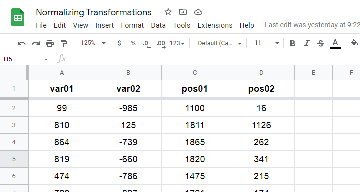
SPSS users may download the exact same data as normalizing-transformations.sav.
Since some transformations don't apply to negative and/or zero values, we “positified” both variables: we added a constant to them such that their minima were both 1, resulting in pos01 and pos02.
Although some transformations could be applied to the original variables, the “normalizing” effects looked very disappointing. We therefore decided to limit this discussion to only our positified variables.
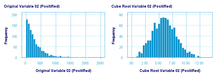
Square/Cube Root Transformation
A cube root transformation did a great job in normalizing our positively skewed variable as shown below.
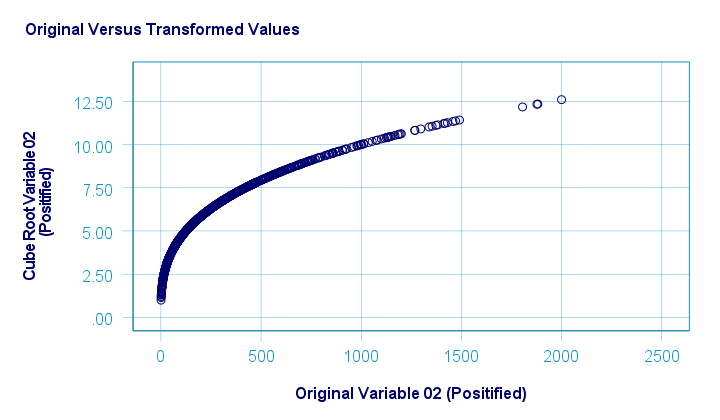
The scatterplot below shows the original versus transformed values.
SPSS refuses to compute cube roots for negative numbers. The syntax below, however, includes a simple workaround for this problem.
compute curt01 = pos01**(1/3).
compute curt02 = pos02**(1/3).
*NOTE: IF VARIABLE MAY CONTAIN NEGATIVE VALUES, USE.
*if(pos01 >= 0) curt01 = pos01**(1/3).
*if(pos01 < 0) curt01 = -abs(pos01)**(1/3).
*HISTOGRAMS.
frequencies curt01 curt02
/format notable
/histogram.
*SCATTERPLOTS.
graph/scatter pos01 with curt01.
graph/scatter pos02 with curt02.
Logarithmic Transformation
A base 10 logarithmic transformation did a decent job in normalizing var02 but not var01. Some results are shown below.
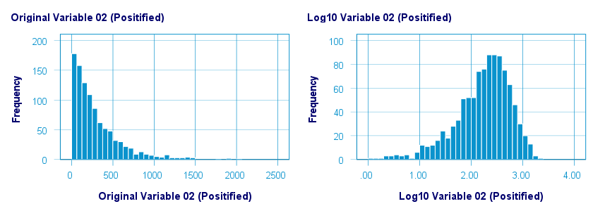
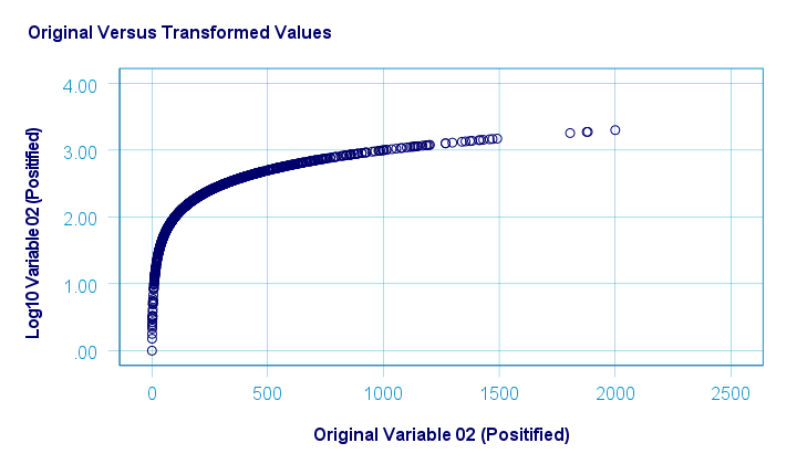
The scatterplot below visualizes the original versus transformed values.
SPSS users can replicate these results from the syntax below.
compute log01 = lg10(pos01).
compute log02 = lg10(pos02).
*HISTOGRAMS.
frequencies log01 log02
/format notable
/histogram.
*SCATTERPLOTS.
graph/scatter pos01 with log01.
graph/scatter pos02 with log02.
Power Transformation
A third power (or cube) transformation was one of the few transformations that had some normalizing effect on our left skewed variable as shown below.
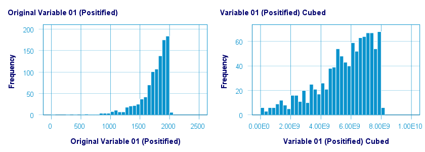
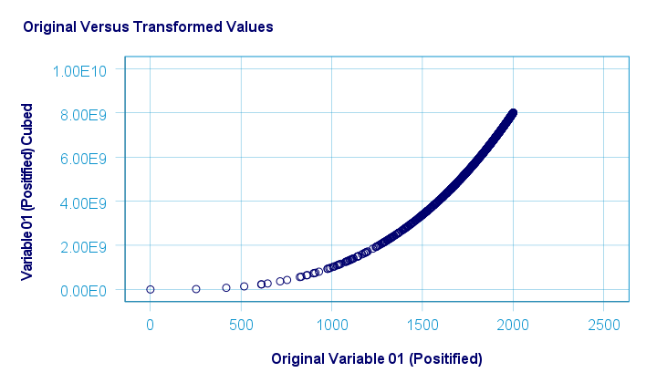
The scatterplot below shows the original versus transformed values for this transformation.
These results can be replicated from the syntax below.
compute cub01 = pos01**3.
compute cub02 = pos02**3.
*HISTOGRAMS.
frequencies cub01 cub02
/format notable
/histogram.
*SCATTERS.
graph/scatter pos01 with cub01.
graph/scatter pos02 with cub02.
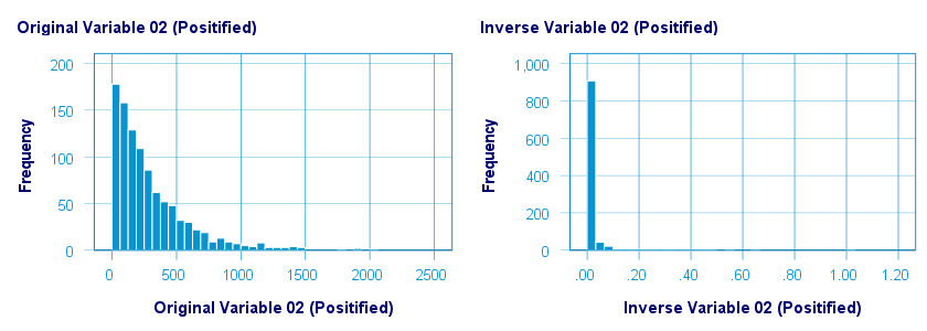
Inverse Transformation
The inverse transformation did a disastrous job with regard to normalizing both variables. The histograms below visualize the distribution for pos02 before and after the transformation.
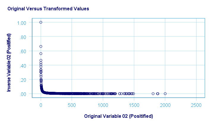
The scatterplot below shows the original versus transformed values. The reason for the extreme pattern in this chart is setting an arbitrary minimum of 1 for this variable as discussed under normalizing negative values.
SPSS users can use the syntax below for replicating these results.
compute inv01 = 1 / pos01.
compute inv02 = 1 / pos02.
*NOTE: IF VARIABLE MAY CONTAIN ZEROES, USE.
*if(pos01 <> 0) inv01 = 1 / pos01.
*HISTOGRAMS.
frequencies inv01 inv02
/format notable
/histogram.
*SCATTERPLOTS.
graph/scatter pos01 with inv01.
graph/scatter pos02 with inv02.
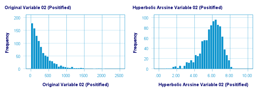
Hyperbolic Arcsine Transformation
As shown below, the hyperbolic arcsine transformation had a reasonably normalizing effect on var02 but not var01.
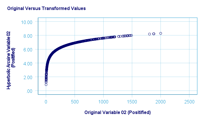
The scatterplot below plots the original versus transformed values.
In Excel and Googlesheets, the hyperbolic arcsine is computed from =ASINH(...) There's no such function in SPSS but a simple workaround is using
$$Asinh_x = ln(Var_x + \sqrt{Var_x^2 + 1})$$
The syntax below does just that.
compute asinh01 = ln(pos01 + sqrt(pos01**2 + 1)).
compute asinh02 = ln(pos02 + sqrt(pos02**2 + 1)).
*HISTOGRAMS.
frequencies asinh01 asinh02
/format notable
/histogram.
*SCATTERS.
graph/scatter pos01 with asinh01.
graph/scatter pos02 with asinh02.
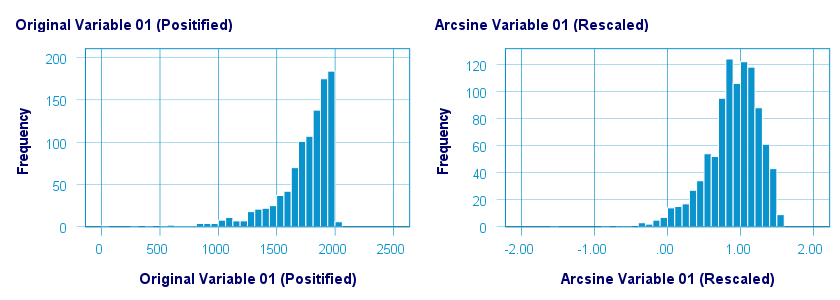
Arcsine Transformation
Before applying the arcsine transformation, we first rescaled both variables to a range of [-1, +1]. After doing so, the arcsine transformation had a slightly normalizing effect on both variables. The figure below shows the result for var01.
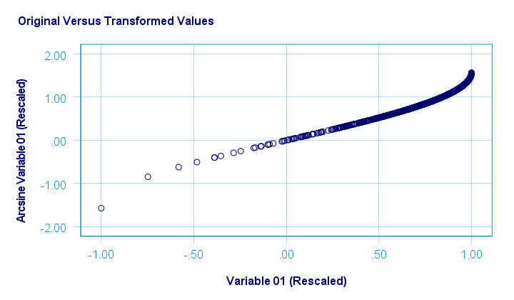
The original versus transformed values are visualized in the scatterplot below.
The rescaling of both variables as well as the actual transformation were done with the SPSS syntax below.
aggregate outfile * mode addvariables
/min01 min02 = min(var01 var02)
/max01 max02 = max(var01 var02).
*RESCALE VARIABLES TO [-1, +1] .
compute trans01 = (var01 - min01)/(max01 - min01)*2 - 1.
compute trans02 = (var02 - min01)/(max01 - min01)*2 - 1.
*ARCSINE TRANSFORMATION.
compute asin01 = arsin(trans01).
compute asin02 = arsin(trans02).
*HISTOGRAMS.
frequencies asin01 asin02
/format notable
/histogram.
*SCATTERS.
graph/scatter trans01 with asin01.
graph/scatter trans02 with asin02.
Descriptives after Transformations
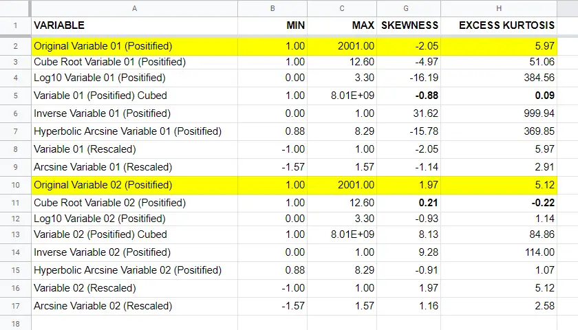
The figure below summarizes some basic descriptive statistics for our original variables before and after all transformations. The entire table is available from this Googlesheet (read-only).
Conclusion
If we only judge by the skewness and kurtosis after each transformation, then for our 2 test variables
- the third power transformation had the strongest normalizing effect on our left skewed variable and
- the cube root transformation worked best for our right skewed variable.
I should add that none of the transformations did a really good job for our left skewed variable, though.
Obviously, these conclusions are based on only 2 test variables. To what extent they generalize to a wider range of data is unclear. But at least we've some idea now.
If you've any remarks or suggestions, please throw us a quick comment below.
Thanks for reading.
THIS TUTORIAL HAS 15 COMMENTS:
By Jon K Peck on February 28th, 2023
Box-Cox is in ADP, which is used by ALM. You can use that by itself.
The extension I am writing is using sklearn. I first started trying to use the R caret package, but I had too many problems with that and discarded it.
If you want to use a Python or R package with Statistics that is not automatically included, you can use the STATS PACKAGE INSTALL extension command to get it, but dependencies declared in an spe file, whether one on the Extension Hub or one you write yourself, will be automatically installed if possible from CRAN or PyPI.
By Priyanka Sanap on March 27th, 2024
The article is full of statistics example with technical information.
By Jon Peck on March 30th, 2025
Why no mention of Box-Cox? Also, Yeo-Johnson is a modified Box-Cox that allows for negative values.
These and others are available in the STATS PREPROCESS extension command.
By Ruben Geert van den Berg on March 31st, 2025
Hi Jon!
Perhaps I should add it but I'm not quite sure.
I kinda feel it's not really part of the mainstream literature.
Few -if any- standard textbooks (for social scientists, that is) even mention it...
By Jon K Peck on March 31st, 2025
My impression is that Box-Cox is actually the most popular normalizing transformation in use - not that I have any real data to back that up. Yeo-Johnson is less well known.