A newly updated, ad-free video version of this tutorial
is included in our SPSS beginners course.
Null Hypothesis for the Chi-Square Independence Test
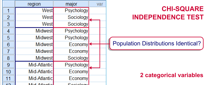
A chi-square independence test evaluates if two categorical variables are associated in some population. We'll therefore try to refute the null hypothesis that
two categorical variables are (perfectly) independent in some population.
If this is true and we draw a sample from this population, then we may see some association between these variables in our sample. This is because samples tend to differ somewhat from the populations from which they're drawn.
However, a strong association between variables is unlikely to occur in a sample if the variables are independent in the entire population. If we do observe this anyway, we'll conclude that the variables probably aren't independent in our population after all. That is, we'll reject the null hypothesis of independence.
Example
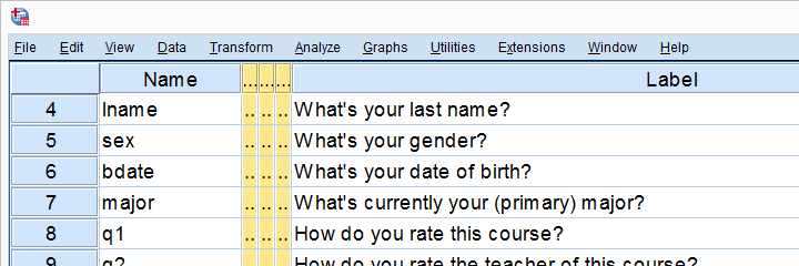
A sample of 183 students evaluated some course. Apart from their evaluations, we also have their genders and study majors. The data are in course_evaluation.sav, part of which is shown below.
We'd now like to know: is study major associated with gender? And -if so- how? Since study major and gender are nominal variables, we'll run a chi-square test to find out.
Assumptions Chi-Square Independence Test
Conclusions from a chi-square independence test can be trusted if two assumptions are met:
- independent observations. This usually -not always- holds if each case in SPSS holds a unique person or other statistical unit. Since this is that case for our data, we'll assume this has been met.
- For a 2 by 2 table, all expected frequencies > 5.If you've no idea what that means, you may consult Chi-Square Independence Test - Quick Introduction. For a larger table, no more than 20% of all cells may have an expected frequency < 5 and all expected frequencies > 1.
SPSS will test this assumption for us when we'll run our test. We'll get to it later.
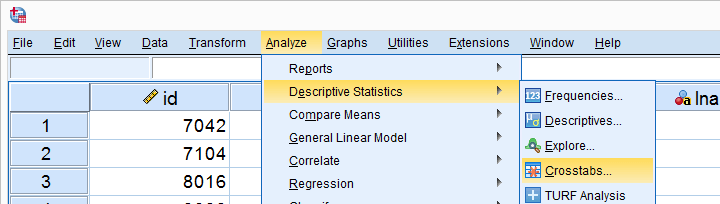
Chi-Square Independence Test in SPSS
In SPSS, the chi-square independence test is part of the CROSSTABS procedure which we can run as shown below.
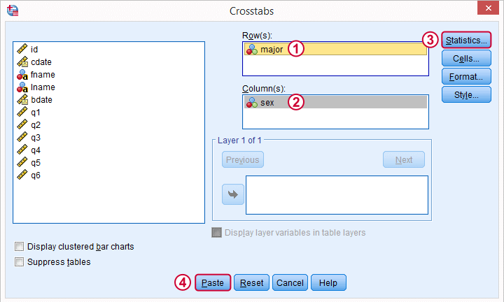
In the main dialog, we'll enter one variable into the box and the other into . Since sex has only 2 categories (male or female), using it as our column variable results in a table that's rather narrow and high. It will fit more easily into our final report than a wider table resulting from using major as our column variable. Anyway, both options yield identical test results.
 Under we'll just select . Clicking results in the syntax below.
SPSS Chi-Square Independence Test Syntax
CROSSTABS
/TABLES=major BY sex
/FORMAT=AVALUE TABLES
/STATISTICS=CHISQ
/CELLS=COUNT
/COUNT ROUND CELL.
You can use this syntax if you like but I personally prefer a shorter version shown below. I simply type it into the Syntax Editor window, which for me is much faster than clicking through the menu. Both versions yield identical results.
crosstabs major by sex
/statistics chisq.
Output Chi-Square Independence Test
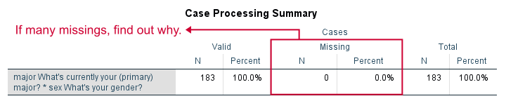
First off, we take a quick look at the Case Processing Summary to see if any cases have been excluded due to missing values. That's not the case here. With other data, if many cases are excluded, we'd like to know why and if it makes sense.
Contingency Table
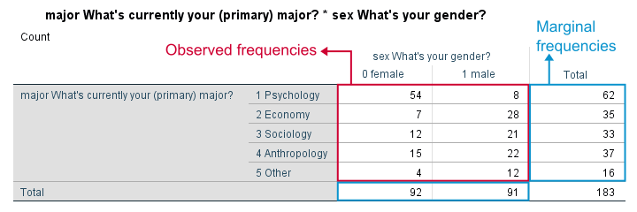
Next, we inspect our contingency table. Note that its marginal frequencies -the frequencies reported in the margins of our table- show the frequency distributions of either variable separately.
Both distributions look plausible and since there's no “no answer” categories, there's no need to specify any user missing values.
Significance Test
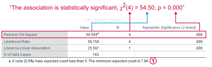
 First off, our data meet the assumption of all expected frequencies > 5 that we mentioned earlier. Since this holds, we can rely on our significance test for which we use Pearson Chi-Square.
Right, we usually say that the association between two variables is statistically significant if Asymptotic Significance (2-sided) < 0.05 which is clearly the case here.
Significance is often referred to as “p”, short for probability; it is the probability of observing our sample outcome if our variables are independent in the entire population. This probability is 0.000 in our case. Conclusion: we reject the null hypothesis that our variables are independent in the entire population.
Understanding the Association Between Variables
We conclude that our variables are associated but what does this association look like? Well, one way to find out is inspecting either column or row percentages. I'll compute them by adding a line to my syntax as shown below.
set tvars labels tnumbers labels.
*Crosstabs with frequencies and row percentages.
crosstabs major by sex
/cells count row
/statistics chisq.
Adjusting Our Table
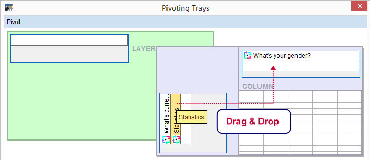
Since I'm not too happy with the format of my newly run table, I'll right-click it and select
![]()
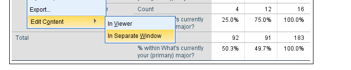
We select and then drag and drop right underneath “What's your gender?”. We'll close the pivot table editor.
Result
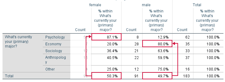
Roughly half of our sample if female. Within psychology, however, a whopping 87% is female. That is, females are highly overrepresented among psychology students. Like so, study major “says something” about gender: if I know somebody studies psychology, I know she's probably female.
The opposite pattern holds for economy students: some 80% of them are male. In short, our row percentages describe the association we established with our chi-square test.
We could quantify the strength of the association by adding Cramér’s V to our test but we'll leave that for another day.
Reporting a Chi-Square Independence Test
We report the significance test with something like “an association between gender and study major was observed, χ2(4) = 54.50, p = 0.000. Further, I suggest including our final contingency table (with frequencies and row percentages) in the report as well as it gives a lot of insight into the nature of the association.
So that's about it for now. Thanks for reading!
THIS TUTORIAL HAS 73 COMMENTS:
By Ruben Geert van den Berg on June 10th, 2016
Hi Saroj!
Supposedly, the adjusted standardized residuals should follow a standard normal distribution. With a reasonable sample size, a rule of thumb is that values < -3 or > 3 are unlikely to occur under the null hypothesis and therefore indicate a deviation thereof. Since this is a somewhat different test than the standard chi-square test, one may be significant while the other isn't or reversely. Statistics really isn't exact science after all.
Right, beware that there's standardized and adjusted standardized residuals and you want to use the latter. I believe you'll get them by adding
ASRESIDtoCELLSas inCROSSTABS DSM BY GENDER/CELLS COUNT ARESID/STATISTICS CHISQ.Hope that helps!
By Saroj on June 10th, 2016
Thanks Ruben
Much appreciated.
By SUNDUS on June 29th, 2016
Excellent!
Just one query. I hope u will clarify it.
"we observed a strong association between the current and the preferred brands, χ2(9) = 131.2, p = .000", but can u tell me how can we comment that which brand of smart phone was the best while discussion in the discussion section. Can we do with in group comparison like ANOVA while using chi-square,
By carla on August 1st, 2016
Hi, this website has helped me greatly. I'm currently running chi-square tests for my masters thesis. Every Asymp.sig is .000 is this wrong? Also, if my variables have more than 2 categories do i still follow the same procedure? Thanks
By Ruben Geert van den Berg on August 2nd, 2016
Hi Carla! With large sample sizes (say n > 200 or so), it's quite normal that basically all chi-square tests yield p < 0.000. However, please keep in mind the exact interpretation of this result: it means that the variables are unlikely to be perfectly unassociated. It does not mean that the association among them is strong. That is, the association is statistically significant but not necessarily practically significant, ok?
Yes, you follow the same procedure when there's more than 2 categories. Do watch out for variables with many (small) categories as they may violate the assumption that all Ei > 5. If this happens, it may be wise to merge some of the smaller categories into a new one called "other" or something.