Using categorical predictors in multiple regression requires dummy coding. So how to use such dummy variables and how to interpret the resulting output? This tutorial walks you through.
- Example I - Single Dummy Predictor
- Example II - Multiple Dummy Predictors
- Example III - Quantitative and Dummy Predictors
- Is Dummy Variable Regression Useless?
Example Data
All examples in this tutorial use staff-dummies.sav, partly shown below.
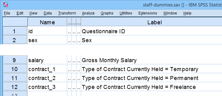
Our data file already contains dummy variables for representing Contract Type. Two options for creating such dummy variables in other data files are
Analysis I - T-Test as Dummy Regression
Let's first examine if monthly salary is related to sex. Two options for finding this out are
- an independent samples t-test or
- simple linear regression with sex as a single dummy predictor.
These analyses come up with the same results. Comparing these is the first step towards understanding dummy variable regression. Let's first run our t-test from the syntax below.
t-test groups sex(1 0)
/variables salary.
Results
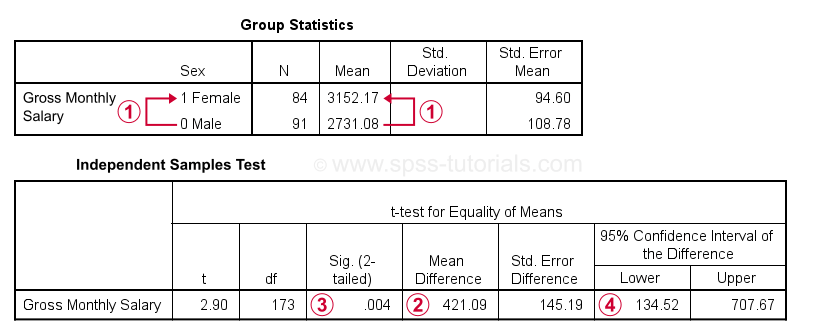
 Gross monthly salary for females is $421.09 higher than for males. Also note that males are coded 0 while females are coded 1.
 The significance level for this mean difference is 0.004: we'll probably reject the null hypothesis that the population mean salaries are equal between men and women.
 A 95% confidence interval suggests a likely range for the population mean difference. It runs from $134.52 through $707.67.
Let's now rerun this analysis as regression with a single dummy variable.
Example I - Single Dummy Predictor
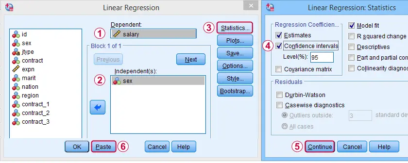
In SPSS, we first navigate to
![]()
![]() and fill out the dialogs as shown below.
and fill out the dialogs as shown below.
Completing these steps results in the syntax below. Let's run it.
REGRESSION
/MISSING LISTWISE
/STATISTICS COEFF OUTS CI(95) R ANOVA
/CRITERIA=PIN(.05) POUT(.10)
/NOORIGIN
/DEPENDENT salary
/METHOD=ENTER sex.
Dummy Variable Regression Output I
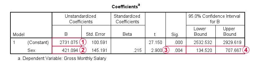
Note that the constant is the mean salary for male respondents.
 The b-coefficient for sex is the mean salary difference between male and female respondents. This is equal to the average increase in salary associated with a 1-unit increase in sex: from male (coded 0) to female (coded 1).
This makes sense because the regression equation is
$$Salary' = $2731 + $421 \cdot Sex$$
so for all males we predict a gross monthly salary of
$$Salary' = $2731 + $421 \cdot 0 = $2731$$
and for all females we predict
$$Salary' = $2731 + $421 \cdot 1 = $3152$$
These predicted salaries are simply the mean salaries for male and female respondents.
Finally, note that the significance level and confidence interval for the b-coefficient are identical to their counterparts for the mean difference in the t-test results.
Analysis II - ANOVA as Dummy Regression
Let's now see if salary is related to contract type (freelance, temporary or permanent). Precisely, we'll test the null hypothesis that the population mean salaries are equal across all 3 contract types. Two options for testing this hypothesis are:
- ANOVA and
- dummy variable regression.
As we'll see, the b-coefficients obtained from our regression approach are identical to simple contrasts from ANOVA: the mean for a designated reference category is compared to the mean for each other category. These ANOVA results can be replicated from the syntax below.
unianova salary by contract
/contrast (contract) = simple(1)
/print descriptive etasq.
Results
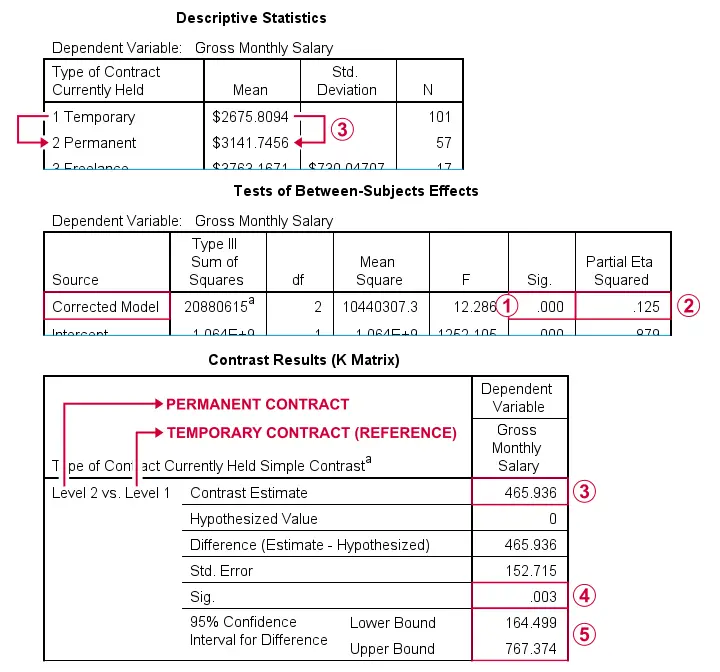
Since p < 0.05, we reject the null hypothesis that all population means are equal.
The effect size, eta squared is 0.125. This is between medium (0.06) and large (0.14).
The mean difference between employees on a permanent versus a temporary contract (the reference category) is $465.94.
The p-value and  confidence interval indicate that this mean difference is “significantly” different from zero, the null hypothesis for this comparison.
In a similar vein, the mean salaries for employees on a freelance versus a temporary contract are compared (not shown here).
Example II - Multiple Dummy Predictors
We'll navigate to
![]()
![]() and fill out the dialogs as shown below.
and fill out the dialogs as shown below.
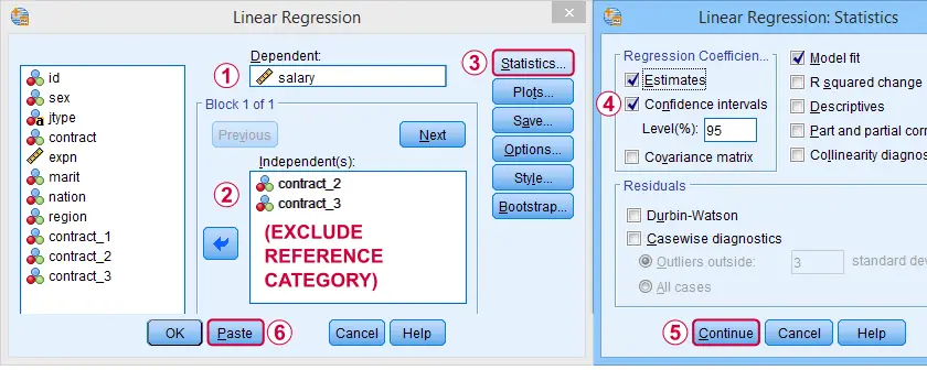
We need to choose one reference category and not enter it as a predictor: for representing k categories, we always enter (k - 1) dummy variables.
 Competing these steps generates the syntax below.
REGRESSION
/MISSING LISTWISE
/STATISTICS COEFF OUTS CI(95) R ANOVA
/CRITERIA=PIN(.05) POUT(.10)
/NOORIGIN
/DEPENDENT salary
/METHOD=ENTER contract_2 contract_3.
Dummy Variable Regression Output II
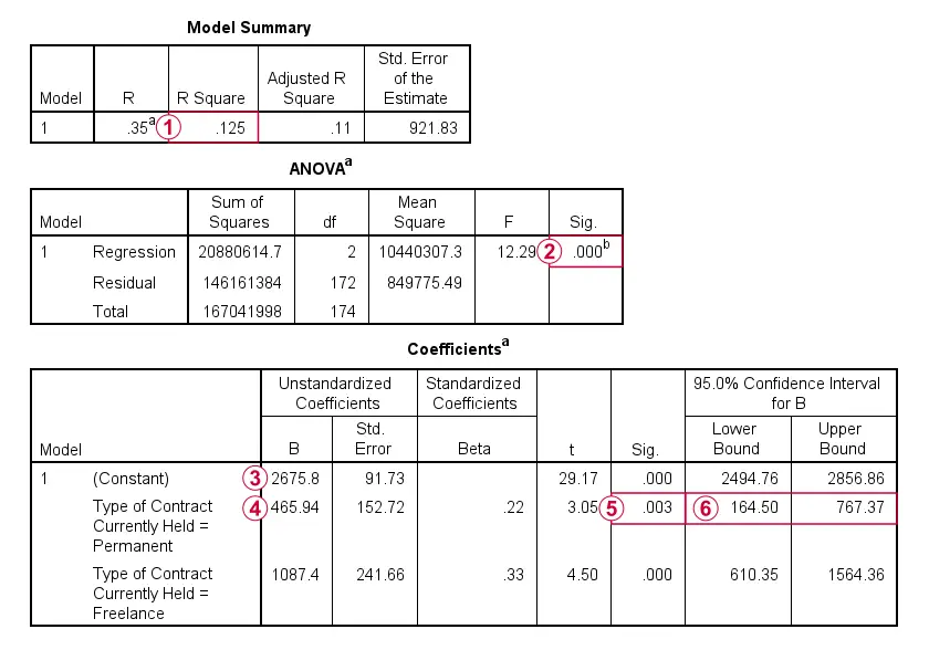
Note that r-squared is equal to the ANOVA eta squared we saw earlier. This is always the case: both measures indicate the proportion of variance in the dependent variable accounted for by the independent variable(s).
R-squared for the entire model (containing only 2 dummy variables) is statistically significant. In fact, the entire regression ANOVA table is identical to the one obtained from an actual ANOVA.
The constant is the mean salary for our reference category: employees having a temporary contract. These respondents score zero on both dummy variables in our model. For them, the regression equation boils down to
$$Salary' = $2675.8 + $465.94 \cdot 0 + $1087.4 \cdot 0 = $2675.8$$
The b-coefficients are the mean differences between each dummy category and the reference category: the mean salary for employees on a permanent contract is $465.94 higher than for those on a temporary contract.
The mean salary difference between permanent and temporary contract employees is “significantly” different from zero because p < 0.05.
All b-coefficients and their p-values and confidence intervals are identical to the simple contrasts we saw in the earlier ANOVA results.
A final point on these results is that you should enter either all or none of the dummy variables representing the same categorical variable. If you don't, then the b-coefficients no longer correspond to the mean differences between dummy categories and the reference category. The figure below attempts to clarify this somewhat challenging point.
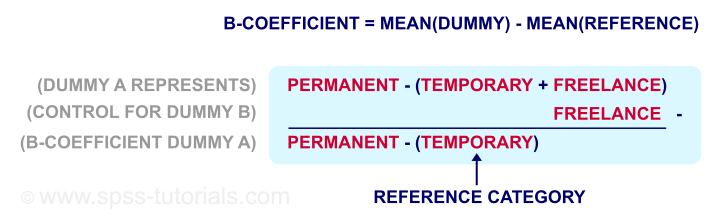
In short, a dummy variable represents some category versus all other categories lumped together. Partialling out these other categories except the reference isolates the effects: this renders the b-coefficients equal to the mean differences between dummy categories versus the reference category.
Analysis III - ANCOVA as Dummy Regression
Thus far, we saw that contract type is associated with mean salary. However, could this be merely due to working experience? Employees having more years on the job get better contract types as well as higher salaries just because they've more experience?
Two options for ruling out such possible confounding out are
- multiple regression analysis with experience and 2 dummy variables for contract type as predictors.
- ANCOVA with job type as a fixed factor and experience as a covariate.
Let's first analyze this as a dummy variable regression. We'll then replicate the results via the ANCOVA approach.
Example III - Quantitative and Dummy Predictors
Again, let's navigate to
![]()
![]() and complete the steps shown below.
and complete the steps shown below.
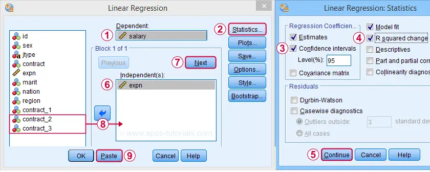
For this example, we'll run a hierachical regression analysis: we first just enter our control variable, expn (working experience).
 We then request a second “Block” of predictors.
 Finally, we enter 2 dummy variables (excluding contract_1, our reference category) as our second block.
 These steps result in the syntax below.
REGRESSION
/MISSING LISTWISE
/STATISTICS COEFF OUTS CI(95) R ANOVA CHANGE
/CRITERIA=PIN(.05) POUT(.10)
/NOORIGIN
/DEPENDENT salary
/METHOD=ENTER expn
/METHOD=ENTER contract_2 contract_3.
Dummy Variable Regression Output III
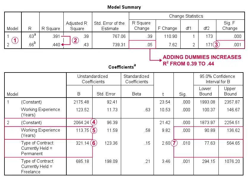
SPSS has run and compared 2 regression models: model 1 contains working experience as the (sole) quantitative predictor. Model 2 adds our 2 dummy variables representing contract type to model 1.
Adding the contract type dummies to working experience increases r-squared from 0.39 to 0.44.
This increase is statistically significant: our dummies contribute to predicting salary over and above just working experience.
The constant in model 2 is the mean salary for employees who are a) on a temporary contract (reference category) and b) have 0 years of working experience. These are employees who score zero on all predictors in model 2.
A 1 unit (year) increase in working experience is associated with an average $113.75 increase in monthly salary if we control for contract type.
The mean salary difference between employees on permanent (dummy) versus temporary (reference) contracts is $321.14 if we control for working experience.
Since p < 0.05, this mean difference is statistically significant.
Let's now rerun the exact same analysis as an ANCOVA from the syntax below.
unianova salary by contract with expn
/contrast (contract) = simple(1)
/print descriptive etasq.
Results
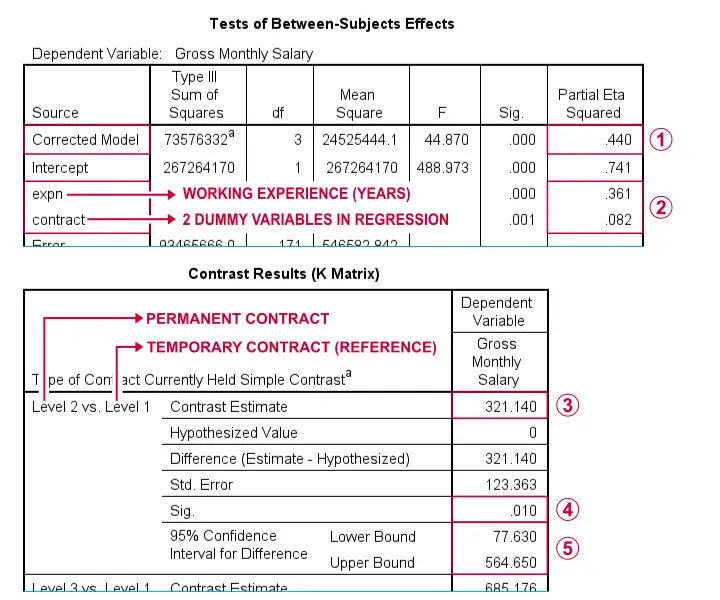
Partial eta squared for “corrected model” is equal to the regression r-squared.
The output also contains effect sizes for both predictors separately. Note that 0.361 and 0.082 add up to 0.443, somewhat larger than 0.440 for the entire model. This is because these effects partially overlap: experience is associated with contract type.
The mean salary difference between employees on permanent versus temporary contracts is $321.14 if we correct for working experience. This difference was seen as a b-coefficient in the previous dummy regression output.
Unsurprisingly, the p-value and confidence interval are identical to their dummy regression counterparts as well.
Is Dummy Variable Regression Useless?
Many textbooks propose dummy variable regression as the only option for using a combination of quantitative and categorical predictors. However, our last example suggests that ANCOVA may be a better option for this scenario. Why? Well,
- ANCOVA does not require adding (technically redundant) dummy variables to your data.
- ANCOVA comes up with a single effect size (partial eta squared) for the entire categorical predictor. This is more useful than effect sizes for separate dummy variables because we never add them separately to a regression model.
- Testing moderation effects between quantitative and categorical predictors is fairly easy via ANCOVA but rather complicated via regression.
Final Notes
First off, note that the analyses in this tutorial skipped some important steps:
- we didn't inspect any frequency distributions to see if our data look plausible;
- we did't see if there's any missing values in our data;
- we didn't evaluate any model assumptions (normality, linearity, and so on).
We encourage you to thoroughly examine such issues whenever you're working on real-world data files.
Right, so that should do for dummy regression in SPSS. For a handy overview of the output from all 6 analyses, click here. Did you find this tutorial (not) helpful? Do you agree or disagree with us? Please let us know by throwing a comment below.
Thanks for reading!
THIS TUTORIAL HAS 9 COMMENTS:
By YY Ma on April 8th, 2021
A very instructive post!
I have learnt much from it.
By DR BODDU NARASIMHULU on April 16th, 2021
Good
By MWETEGYEREZE FRANK on May 1st, 2021
It's really interesting
By N M on May 18th, 2021
Thank you so much.Been looking high and low to figure out dummy variable regression interpretation. So would you say that in regression its ideally best not to add multiple categorical variables in the same model?
By Does Malicha Kalicha on July 13th, 2022
It good description of statistics, thank you for all.