• Repeated Measures ANOVA - Null Hypothesis
• Repeated Measures ANOVA - Assumptions
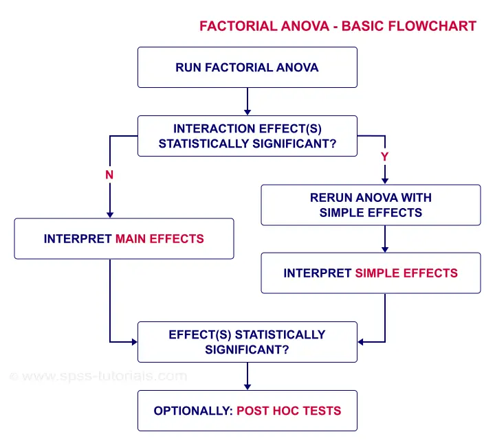
• Factorial ANOVA - Basic Flowchart
• Factorial Repeated Measures ANOVA in SPSS
• Repeated Measures ANOVA - APA Style Reporting

How does alcohol consumption affect driving performance? A study tested 36 participants during 3 conditions:

• no alcohol - 0 glasses of beer;
• medium alcohol - 2 glasses of beer;
• high alcohol - 4 glasses of beer.

Each participant went through all 3 conditions in random order on 3 consecutive days. During each condition, the participants drove for 30 minutes in a driving simulator. During these “rides” they were confronted with 5 trials: dangerous situations to which they need to respond fast. The 15 reaction times (5 trials for each of 3 conditions) are in alcoholtest.sav, part of which is shown below.

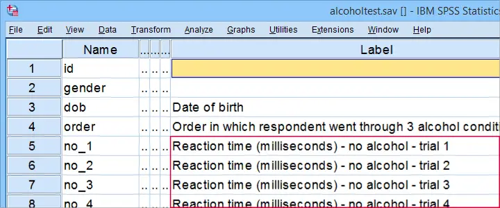
The main research questions are

• how does alcohol affect reaction times?
• how does trial affect reaction times?
• does the effect of alcohol depend on trial?

We'll obviously inspect the mean reaction times over (combinations of) conditions and trials. However, we've only 36 participants. Based on this tiny sample, what -if anything- can we conclude about the general population? The right way to answer that is running a repeated measures ANOVA over our 15 reaction time variables.

Repeated Measures ANOVA - Null Hypothesis

Generally, the null hypothesis for a repeated measures ANOVA is that the population means of 3+ variables are all equal. If this is true, then the corresponding sample means may differ somewhat. However, very different sample means are unlikely if population means are equal. So if that happens, we no longer believe that the population means were truly equal: we reject this null hypothesis.

Now, with 2 factors -condition and trial- our means may be affected by condition, trial or the combination of condition and trial: an interaction effect. We'll examine each of these possible effect separately. This means we'll test 3 null hypotheses:

• population means are equal over conditions;
• population means are equal over trials;
• population means are equal over combinations of condition and trial.

As we're about to see: we may or may not reject each of our 3 hypotheses independently of the others.

Repeated Measures ANOVA - Assumptions

A repeated measures ANOVA will usually run just fine in SPSS. However, we can only trust the results if we meet some assumptions. These are:

1. Independent observations or -precisely- independent and identically distributed variables.
2. Normality: the test variables follow a multivariate normal distribution in the population. This is only needed for small sample sizes of N < 25 or so. You can test if variables are normally distributed with a Kolmogorov-Smirnov test or a Shapiro-Wilk test.
3. Sphericity: the population variances of all difference scores among the test variables must be equal. Sphericity is often tested with Mauchly’s test.

With regard to our example data in alcoholtest.sav:

1. Independent observations is probably met: each case contains a separate person who didn't interact in any way with any other participants.
2. We don't need normality because we've a reasonable sample size of N = 36.
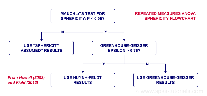
3. We'll use Mauchly's test to see if sphericity is met. If it isn't, we'll apply a correction to our results as shown in our sphericity flowchart.

Data Checks I - Histograms

Let's first see if our data look plausible in the first place. Since our 15 reaction times are quantitative variables, running some basic histograms over them will give us some quick insights. The fastest way to do so is running the syntax below. Easier -but slower- alternatives are covered in Creating Histograms in SPSS.

I won't bother you with the output. See for yourself that all frequency distributions look at least reasonably plausible.

Data Checks II - Missing Values

In SPSS, repeated measures ANOVA uses
only cases without any missing values on any of the test variables. That's right: cases having one or more missing values on the 15 reaction times are completely excluded from the analysis. This is a major pitfall and it's hard to detect after running the analysis.

Our advice is to inspect how many cases are complete on all test variables before running the actual analysis. A very fast way to do so is running a minimal DESCRIPTIVES table.

Result

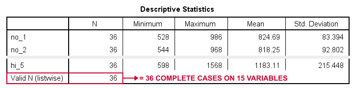
“Valid N (listwise)” indicates the number of cases who are complete on all variables in this table. For our example data, all 36 cases are complete. All cases will be used for our repeated measures ANOVA.

If missing values do occur in other data, you may want to exclude such cases altogether before proceeding. The simplest options are FILTER or SELECT IF. Alternatively, you could try and impute some -or all- missing values.

Creating a Reporting Table

Our last step before the actual ANOVA is creating a table with descriptive statistics for reporting. The APA suggests using 1 row per variable that includes something like

• sample size;
• mean;
• 95% confidence interval for the mean;
• median;
• standard deviation and
• skewness.

A minimal EXAMINE table comes close:

Sadly, there's some issues with EXAMINE that you must know:

• by default, EXAMINE uses only cases that are complete on all variables in the table. We usually don't want that. However, for this example it's great because our final ANOVA is also restricted to complete cases.
• EXAMINE only reports sample sizes in a separate table. This is utter stupidity. However, for this example it's ok: we know we've 36 complete cases. We'll report this in the table title.
• EXAMINE creates way more output than you need and you can't choose which statistics you'll get in which order. The least cumbersome solution is editing the table in Excel.

After creating the table, we'll rearrange its dimensions like we did in SPSS Correlations in APA Format. The result is shown below.

Reporting Table - Result

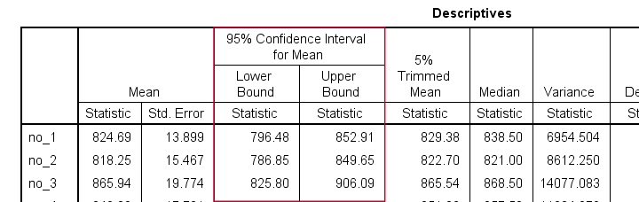
This table contains all descriptives we'd like to report. Moreover, it also allows us to double-check some of the later ANOVA output.

Factorial ANOVA - Basic Flowchart

Factorial Repeated Measures ANOVA in SPSS

The screenshots below guide you through running the actual ANOVA. Note that you'll only have Repeated Measures in your menu if you're licensed for the Advanced Statistics module.

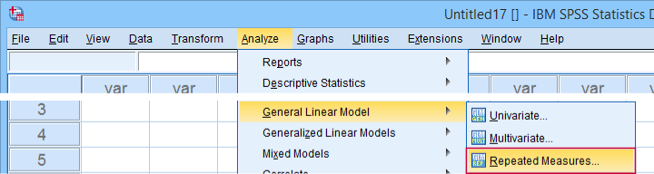
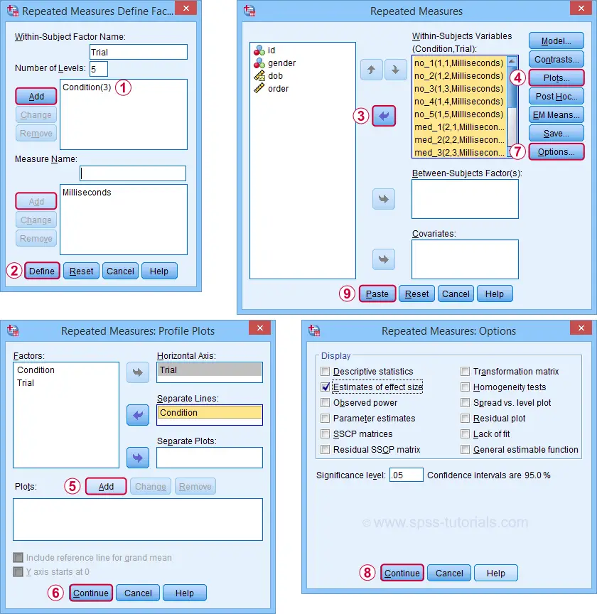
Completing these steps results in the syntax below. Let's run it.

ANOVA Results I - Mauchly's Test

As indicated by our flowchart, we first inspect the interaction effect: condition by trial. Before looking up its significance level, let's first see if sphericity holds for this effect. We find this in the “Mauchly's Test of Sphericity” table shown below.

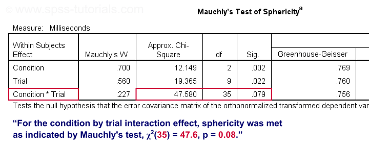
As a rule of thumb, we reject the null hypothesis if p < 0.05. For the interaction effect, “Sig.” or p = 0.079. We retain the null hypothesis. For Mauchly's test, the null hypothesis is that sphericity holds. Conclusion: the sphericity assumption seems to be met. Let's now see if the interaction effect is statistically significant.

ANOVA Results II - Within-Subjects Effects

In the Tests of Within-Subjects Effects table, each effect has 4 rows. We just saw that sphericity holds for the condition by trial interaction. We therefore only use the rows labeled “Sphericity Assumed” as shown below.

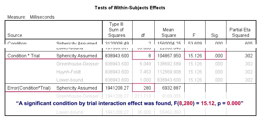
First off, “Sig.” or p = 0.000: the interaction effect is extremely statistically significant. Also note that its effect size -partial eta squared- is 0.302. This indicates a strong effect for condition by trial. But what does that mean? The best way to find out is inspecting our profile plot.

ANOVA Results III - Profile Plot

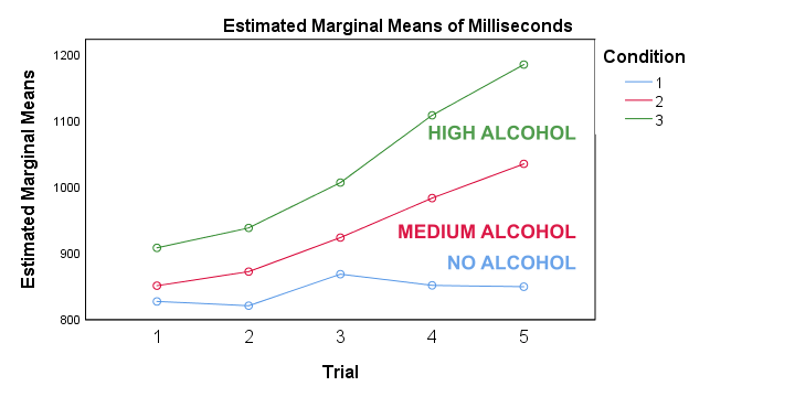
First off, the “estimated marginal means” are simply the observed sample means when running the full factorial model -the default in SPSS. If you're not sure, you can verify this from the reporting table we created earlier. Anyway, what we see is that

• reaction times don't clearly increase over trials for the no alcohol condition;
• reaction times somewhat increase over trials after medium alcohol consumption and
• reaction times strongly increase in the high alcohol condition.

In short, the interaction effect means that the effect of alcohol depends on trial. For the first trial, the lines -representing alcohol conditions- lie close together. But over trials, they diverge further and further. The largest effect of alcohol is seen for trial 5: the reaction times run from 850 milliseconds (no alcohol) up to some 1,200 milliseconds (high alcohol). This implies that there's no such thing as the effect of alcohol. It depends on which trial we inspect. So the logical thing to do is analyze the effect of alcohol for each trial separately. Precisely this is meant by the simple effects suggested in our flowchart.

Rerunning the ANOVA with Simple Effects

So how to run simple effects? It really is simple: we run a one-way repeated measures ANOVA over the 3 conditions for trial 1 only. We'll then just repeat that for trials 2 through 5.
We'll include post hoc tests too. Surprisingly, the Post Hoc dialog is only for between-subjects factors -which we don't have now. For within-subjects factors, use the EM Means dialog as shown below.

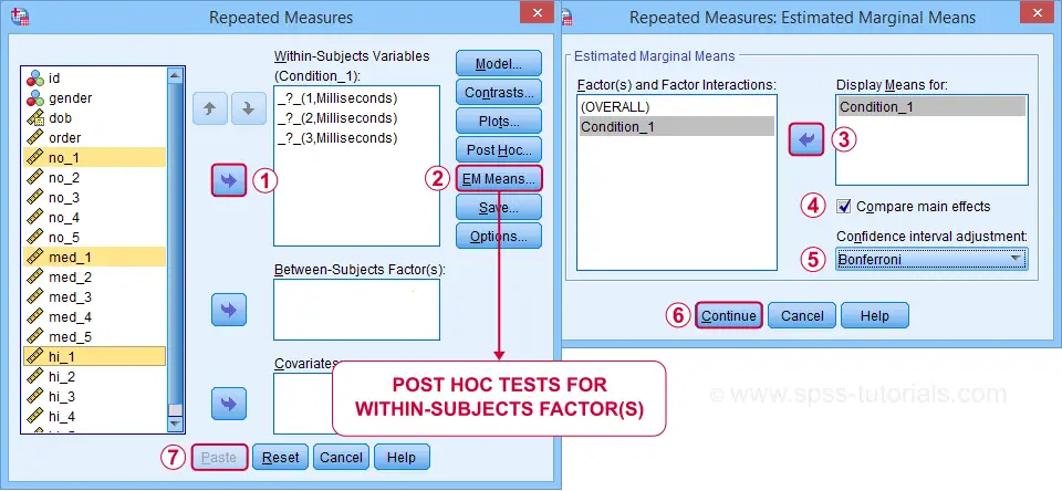
Completing these steps results in the syntax below.

Simple Effects Output I - Mauchly's Test

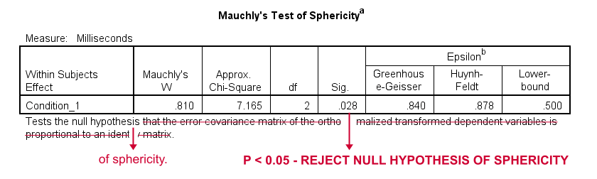
When comparing the 3 alcohol conditions for trial 1 only, Mauchly's test suggests that the sphericity assumption is violated. In this case, we report either

• the Greenhouse-Geisser corrected results or
• the Huyn-Feldt corrected results.

Precisely which depends on the Greenhouse-Geisser epsilon. Epsilon is the Greek letter e written as ε. It estimates to which extent sphericity holds. For this example, ε = 0.840 -a modest violation of sphericity. If ε > 0.75, we report the Huyn-Feldt corrected results as shown below.

Repeated Measures ANOVA - Sphericity Flowchart

Simple Effects Output II - Within-Subjects Effects

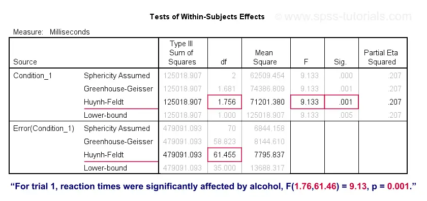
For trial 1, the 3 mean reaction times are significantly different because “Sig.” or p < 0.05. However, note that the effect size -partial eta squared- is modest: η² = 0.207.
In any case, we conclude that the 3 means are not all equal. However, we don't know precisely which means are (not) different. As suggested by our flowchart, we can find out from the post hoc tests we ran.

Simple Effects Output III - Post Hoc Tests

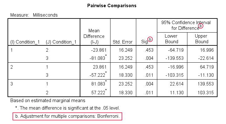
Precisely which means are (not) different? The Pairwise Comparisons table tells us that only the mean difference between conditions 1 and 2
is not statistically significant. So how do these tests work? What SPSS does here, is simply running a paired samples t-test between each pair of variables. For 3 conditions, this results in 3 such tests. Now, 3 tests have a bigger chance of coming up with a false result than 1 test. In order to correct for this, all p-values are multiplied by 3. This is the Bonferroni correction mentioned in the table comment. You can easily verify this by running T-TEST PAIRS=no_1 med_1 hi_1. This results in uncorrected p-values which are equal to the corrected p-values divided by 3.

So that'll do for trial 1. Analyzing trials 2-5 is left as an exercise to the reader.

Repeated Measures ANOVA - APA Style Reporting

First and foremost, present a table with descriptive statistics like the reporting table we created earlier.

Second, report the outcome of Mauchly's test for each effect you discuss: “for trial 1, Mauchly's test indicated a violation
of the sphericity assumption, χ²(2) = 7.17, p = 0.028.”
If sphericity is violated, report the Greenhouse-Geisser ε and which corrected results you'll report: “Since sphericity is violated (ε = 0.840),
Huyn-Feldt corrected results are reported.”
Finally, report the (corrected) F-test results for the within-subjects effects: “Mean reaction times were affected by alcohol,
F(1.76,61.46) = 9.13, p = 0.001, η² = 0.21.”
Note that η² refers to (partial) eta squared, an effect size measure for ANOVA.

Thanks for reading.