A paired samples t-test examines if 2 variables
are likely to have equal population means.

• Paired Samples T-Test Assumptions
• SPSS Paired Samples T-Test Dialogs
• Paired Samples T-Test Output
• Effect Size - Cohen’s D
• Testing the Normality Assumption

Example

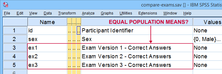
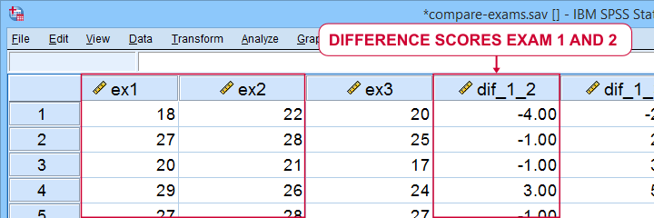
A teacher developed 3 exams for the same course. He needs to know if they're equally difficult so he asks his students to complete all 3 exams in random order. Only 19 students volunteer. Their data -partly shown below- are in compare-exams.sav. They hold the number of correct answers for each student on all 3 exams.

Null Hypothesis

Generally, the null hypothesis for a paired samples t-test is that 2 variables have equal population means. Now, we don't have data on the entire student population. We only have a sample of N = 19 students and sample outcomes tend to differ from population outcomes. So even if the population means are really equal, our sample means may differ a bit. However, very different sample means are unlikely and thus suggest that the population means aren't equal after all. So are the sample means different enough to draw this conclusion? We'll answer just that by running a paired samples t-test on each pair of exams. However, this test requires some assumptions so let's look into those first.

Paired Samples T-Test Assumptions

Technically, a paired samples t-test is equivalent to a one sample t-test on difference scores. It therefore requires the same 2 assumptions. These are

1. independent observations;
2. normality: the difference scores must be normally distributed in the population. Normality is only needed for small sample sizes, say N < 25 or so.

Our exam data probably hold independent observations: each case holds a separate student who didn't interact with the other students while completing the exams.
Since we've only N = 19 students, we do require the normality assumption. The only way to look into this is actually computing the difference scores between each pair of examns as new variables in our data. We'll do so later on.

At this point, you should carefully inspect your data. At the very least, run some histograms over the outcome variables and see if these look plausible. If necessary, set and count missing values for each variable as well. If all is good, proceed with the actual tests as shown below.

SPSS Paired Samples T-Test Dialogs

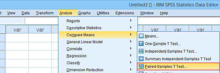
You find the paired samples t-test under Analyze Compare Means Paired Samples T Test as shown below.

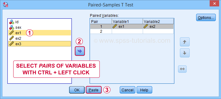
In the dialog below, select each pair of variables and move it to “Paired Variables”. For 3 pairs of variables, you need to do this 3 times.

Clicking Paste creates the syntax below. We added a shorter alternative to the pasted syntax for which you can bypass the entire dialog. Let's run either version.

Paired Samples T-Test Syntax

Paired Samples T-Test Output

SPSS creates 3 output tables when running the test. The last one -Paired Samples Test- shows the actual test results.

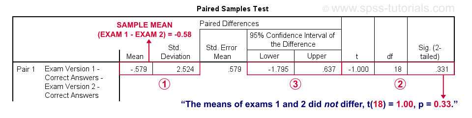
SPSS reports the mean and standard deviation of the difference scores for each pair of variables. The mean is the difference between the sample means. It should be close to zero if the populations means are equal.
The mean difference between exams 1 and 2 is not statistically significant at α = 0.05. This is because ‘Sig. (2-tailed)’ or p > 0.05.
The 95% confidence interval includes zero: a zero mean difference is well within the range of likely population outcomes.

In a similar vein, the second test (not shown) indicates that the means for exams 1 and 3 do differ statistically significantly, t(18) = 2.46, p = 0.025. The same goes for the final test between exams 2 and 3.

Effect Size - Cohen’s D

Our t-tests show that exam 3 has a lower mean score than the other 2 exams. The next question is: are the differences large or small? One way to answer this is computing an effect size measure. For t-tests, Cohen’s D is often used. Sadly, SPSS 27 is the only version that includes it. However, it's easily computed in Excel as shown below.

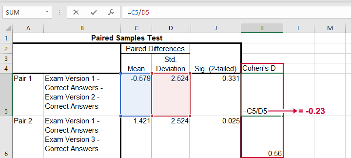
The effect sizes thus obtained are

• d = -0.23 (pair 1) - roughly a small effect;
• d = 0.56 (pair 2) - slightly over a medium effect;
• d = 0.57 (pair 3) - slightly over a medium effect.

Interpretational Issues

Thus far, we compared 3 pairs of exams using 3 t-tests. A shortcoming here is that all 3 tests use the same tiny student sample. This increases the risk that at least 1 test is statistically significant just by chance. There's 2 basic solutions for this:

• apply a Bonferroni correction in order to adjust the significance levels;
• run a repeated measures ANOVA on all 3 exams simultaneously.

If you choose the ANOVA approach, you may want to follow it up with post hoc tests. And these are -guess what?- Bonferroni corrected t-tests again...

Testing the Normality Assumption

Thus far, we blindly assumed that the normality assumption for our paired samples t-tests holds. Since we've a small sample of N = 19 students, we do need this assumption. The only way to evaluate it, is computing the actual difference scores as new variables in our data. We'll do so with the syntax below.

Result

We can now test the normality assumption by running

• a Shapiro-Wilk test or
• a Kolmogorov-Smirnov test.

on our newly created difference scores. Since we discussed both tests in separate tutorials, we'll limit ourselves to the syntax below.

Result

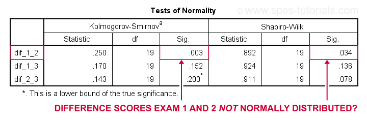
Conclusion: the difference scores between exams 1 and 2 are unlikely to be normally distributed in the population. This violates the normality assumption required by our t-test. This implies that we should perhaps not run a t-test at all on exams 1 and 2. A good alternative for comparing these variables is a Wilcoxon signed-ranks test as this doesn't require any normality assumption.

Last, if you compute difference scores, you can circumvent the paired samples t-tests altogether: instead, you can run one-sample t-tests on the difference scores with zeroes as test values. The syntax below does just that. If you run it, you'll get the exact same results as from the previous paired samples tests.

Right, so that'll do for today. Hope you found this tutorial helpful. And as always:

thanks for reading!