- Shapiro-Wilk Test - What is It?
- Shapiro-Wilk Test - Null Hypothesis
- Running the Shapiro-Wilk Test in SPSS
- Shapiro-Wilk Test - Interpretation
- Reporting a Shapiro-Wilk Test in APA style
Shapiro-Wilk Test - What is It?
The Shapiro-Wilk test examines if a variable
is normally distributed in some population.
Like so, the Shapiro-Wilk serves the exact same purpose as the Kolmogorov-Smirnov test. Some statisticians claim the latter is worse due to its lower statistical power. Others disagree.
As an example of a Shapiro-Wilk test, let's say a scientist claims that the reaction times of all people -a population- on some task are normally distributed. He draws a random sample of N = 233 people and measures their reaction times. A histogram of the results is shown below.
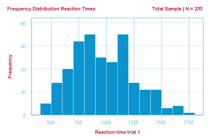
This frequency distribution seems somewhat bimodal. Other than that, it looks reasonably -but not exactly- normal. However, sample outcomes usually differ from their population counterparts. The big question is:
how likely is the observed distribution if the reaction times
are exactly normally distributed in the entire population?
The Shapiro-Wilk test answers precisely that.
How Does the Shapiro-Wilk Test Work?
A technically correct explanation is given on this Wikipedia page. However, a simpler -but not technically correct- explanation is this: the Shapiro-Wilk test first quantifies the similarity between the observed and normal distributions as a single number: it superimposes a normal curve over the observed distribution as shown below. It then computes which percentage of our sample overlaps with it: a similarity percentage.
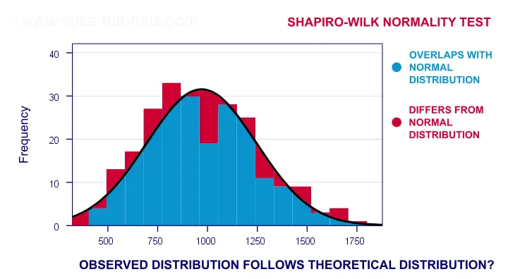
Finally, the Shapiro-Wilk test computes the probability of finding this observed -or a smaller- similarity percentage. It does so under the assumption that the population distribution is exactly normal: the null hypothesis.
Shapiro-Wilk Test - Null Hypothesis
The null hypothesis for the Shapiro-Wilk test is that a variable is normally distributed in some population.
A different way to say the same is that a variable’s values are a simple random sample from a normal distribution. As a rule of thumb, we
reject the null hypothesis if p < 0.05.
So in this case we conclude that our variable is not normally distributed.
Why? Well, p is basically the probability of finding our data if the null hypothesis is true. If this probability is (very) small -but we found our data anyway- then the null hypothesis was probably wrong.
Shapiro-Wilk Test - SPSS Example Data
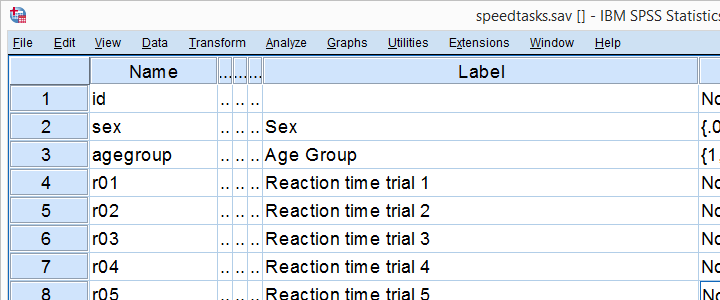
A sample of N = 236 people completed a number of speedtasks. Their reaction times are in speedtasks.sav, partly shown below. We'll only use the first five trials in variables r01 through r05.
I recommend you always thoroughly inspect all variables you'd like to analyze. Since our reaction times in milliseconds are quantitative variables, we'll run some quick histograms over them. I prefer doing so from the short syntax below. Easier -but slower- methods are covered in Creating Histograms in SPSS.
frequencies r01 to r05
/format notable
/histogram normal.
Results
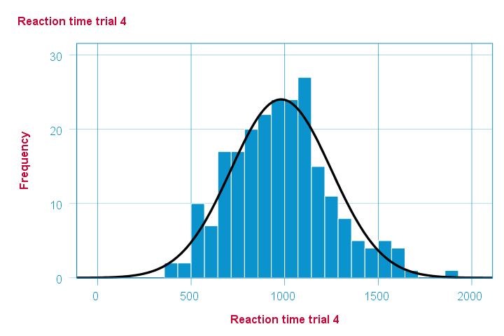
Note that some of the 5 histograms look messed up. Some data seem corrupted and had better not be seriously analyzed. An exception is trial 4 (shown below) which looks plausible -even reasonably normally distributed.
Descriptive Statistics - Skewness & Kurtosis
If you're reading this to complete some assignment, you're probably asked to report some descriptive statistics for some variables. These often include the median, standard deviation, skewness and kurtosis. Why? Well, for a normal distribution,
- skewness = 0: it's absolutely symmetrical and
- kurtosis = 0 too: it's neither peaked (“leptokurtic”) nor flattened (“platykurtic”).
So if we sample many values from such a distribution, the resulting variable should have both skewness and kurtosis close to zero. You can get such statistics from FREQUENCIES but I prefer using MEANS: it results in the best table format and its syntax is short and simple.
means r01 to r05
/cells count mean median stddev skew kurt.
*Optionally: transpose table (requires SPSS 22 or higher).
output modify
/select tables
/if instances = last /*process last table in output, whatever it is...
/table transpose = yes.
Results
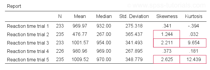
Trials 2, 3 and 5 all have a huge skewness and/or kurtosis. This suggests that they are not normally distributed in the entire population. Skewness and kurtosis are closer to zero for trials 1 and 4.
So now that we've a basic idea what our data look like, let's proceed with the actual test.
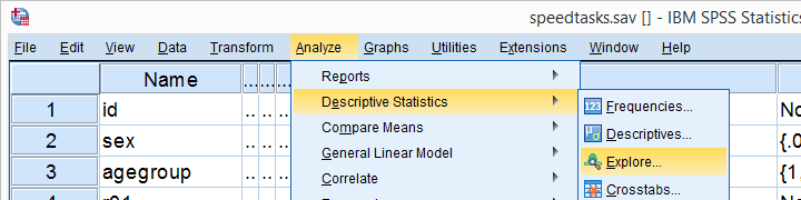
Running the Shapiro-Wilk Test in SPSS
The screenshots below guide you through running a Shapiro-Wilk test correctly in SPSS. We'll add the resulting syntax as well.
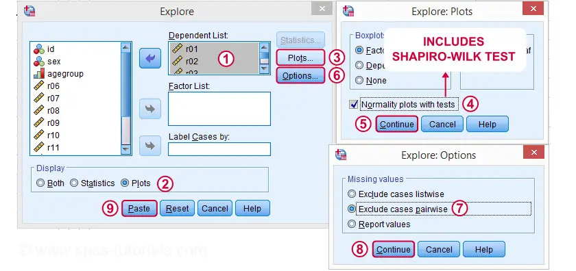
Following these screenshots results in the syntax below.
EXAMINE VARIABLES=r01 r02 r03 r04 r05
/PLOT BOXPLOT NPPLOT
/COMPARE GROUPS
/STATISTICS DESCRIPTIVES
/CINTERVAL 95
/MISSING PAIRWISE /*IMPORTANT!
/NOTOTAL.
Running this syntax creates a bunch of output. However, the one table we're looking for -“Tests of Normality”- is shown below.
Shapiro-Wilk Test - Interpretation
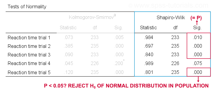
We reject the null hypotheses of normal population distributions
for trials 1, 2, 3 and 5 at α = 0.05.
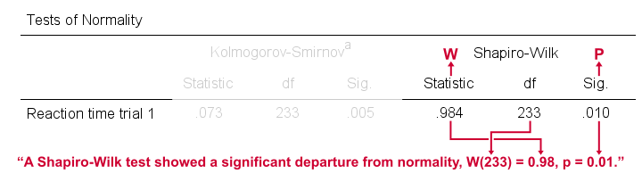
“Sig.” or p is the probability of finding the observed -or a larger- deviation from normality in our sample if the distribution is exactly normal in our population. If trial 1 is normally distributed in the population, there's a mere 0.01 -or 1%- chance of finding these sample data. These values are unlikely to have been sampled from a normal distribution. So the population distribution probably wasn't normal after all.
We therefore reject this null hypothesis. Conclusion: trials 1, 2, 3 and 5 are probably not normally distributed in the population.
The only exception is trial 4: if this variable is normally distributed in the population, there's a 0.075 -or 7.5%- chance of finding the nonnormality observed in our data. That is, there's a reasonable chance that this nonnormality is solely due to sampling error. So
for trial 4, we retain the null hypothesis
of population normality because p > 0.05.
We can't tell for sure if the population distribution is normal. But given these data, we'll believe it. For now anyway.
Reporting a Shapiro-Wilk Test in APA style
For reporting a Shapiro-Wilk test in APA style, we include 3 numbers:
- the test statistic W -mislabeled “Statistic” in SPSS;
- its associated df -short for degrees of freedom and
- its significance level p -labeled “Sig.” in SPSS.
The screenshot shows how to put these numbers together for trial 1.
Limited Usefulness of Normality Tests
The Shapiro-Wilk and Kolmogorov-Smirnov test both examine if a variable is normally distributed in some population. But why even bother? Well, that's because many statistical tests -including ANOVA, t-tests and regression- require the normality assumption: variables must be normally distributed in the population. However,
the normality assumption is only needed for small sample sizes
of -say- N ≤ 20 or so. For larger sample sizes, the sampling distribution of the mean is always normal, regardless how values are distributed in the population. This phenomenon is known as the central limit theorem. And the consequence is that many test results are unaffected by even severe violations of normality.
So if sample sizes are reasonable, normality tests are often pointless. Sadly, few statistics instructors seem to be aware of this and still bother students with such tests. And that's why I wrote this tutorial anyway.
Hey! But what if sample sizes are small, say N < 20 or so? Well, in that case, many tests do require normally distributed variables. However, normality tests typically have low power in small sample sizes. As a consequence, even substantial deviations from normality may not be statistically significant. So when you really need normality, normality tests are unlikely to detect that it's actually violated. Which renders them pretty useless.
Thanks for reading.
THIS TUTORIAL HAS 27 COMMENTS:
By Amrisha on July 28th, 2021
Hi Ruben,
I definitely didn't look at it close enough, haha. Sorry about that. I'd also like to thank you for this tutorial. I've been struggling with using SPSS and was unable to find an easy and accessible explanation for certain concepts. Your tutorial has helped me greatly! Thank you so much once again.
By Ruben Geert van den Berg on July 29th, 2021
That's ok, happens to everybody (including us) sometimes.
Thanks for the compliments and keep up the good work!
SPSS tutorials
By Dr Sciddhartha Koonwar on September 28th, 2021
Was expecting in a totally layman's language.
By Lars-Olov on December 16th, 2021
Tanks - your conclusion was spot on!
By Achar Zachaus Ogutu on December 20th, 2021
My supervisor insisted on a normality test and normally distributed data results ,I had a sample of 384, thanks for this article. I am going to share