A large bank wants to gain insight into their employees’ job satisfaction. They carried out a survey, the results of which are in bank_clean.sav. The survey included some statements regarding job satisfaction, some of which are shown below.
Research Question
The main research question for today is which factors contribute (most) to overall job satisfaction? as measured by overall (“I'm happy with my job”). The usual approach for answering this is predicting job satisfaction from these factors with multiple linear regression analysis.2,6 This tutorial will explain and demonstrate each step involved and we encourage you to run these steps yourself by downloading the data file.
Data Check 1 - Coding
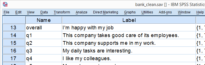
One of the best SPSS practices is making sure you've an idea of what's in your data before running any analyses on them. Our analysis will use overall through q9 and their variable labels tell us what they mean. Now, if we look at these variables in data view, we see they contain values 1 through 11.
So what do these values mean and -importantly- is this the same for all variables? A great way to find out is running the syntax below.
display dictionary
/variables overall to q9.
Result
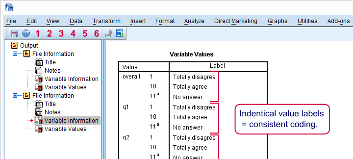
If we quickly inspect these tables, we see two important things:
- for all statements, higher values indicate stronger agreement;
- all statements are positive (“like” rather than “dislike”): more agreement indicates more positive sentiment.
Taking these findings together, we expect positive (rather than negative) correlations among all these variables. We'll see in a minute that our data confirm this.
Data Check 2 - Distributions
Our previous table suggests that all variables hold values 1 through 11 and 11 (“No answer”) has already been set as a user missing value. Now let's see if the distributions for these variables make sense by running some histograms over them.
frequencies overall to q9
/format notable
/histogram.
Data Check 3 - Missing Values
First and foremost, the distributions of all variables show values 1 through 10 and they look plausible. However, we have 464 cases in total but our histograms show slightly lower sample sizes. This is due to missing values. To get a quick idea to what extent values are missing, we'll run a quick DESCRIPTIVES table over them.
set tvars labels.
*2. Check for missings and listwise valid n.
descriptives overall to q9.
Result
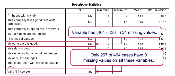
For now, we mostly look at N, the number of valid values for each variable. We see two important things:
- The lowest N is 430 (“My workspace is good”) out of 464 cases; roughly 7% of the values are missing.
- Only 297 cases have zero missing values on all variables in this table.
Correlations
We'll now inspect the correlations over our variables as shown below.
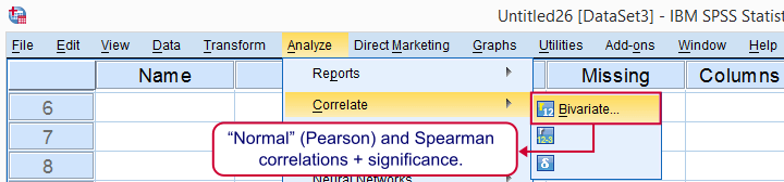
In the next dialog, we select all relevant variables and leave everything else as-is. We then click , resulting in the syntax below.
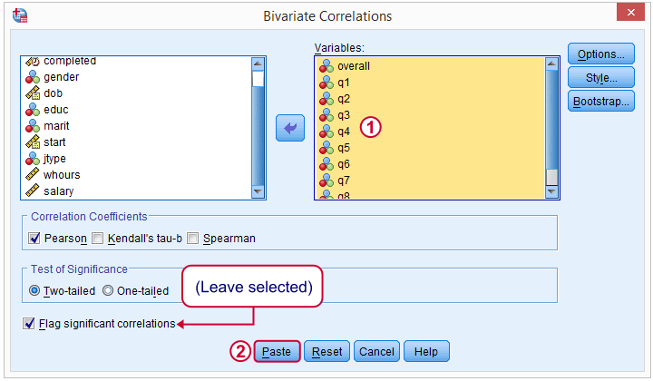
CORRELATIONS
/VARIABLES=overall q1 q2 q3 q4 q5 q6 q7 q8 q9
/PRINT=TWOTAIL NOSIG
/MISSING=PAIRWISE.
Importantly, note the last line -/MISSING=PAIRWISE.- here.
Result
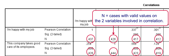
Note that all correlations are positive -like we expected. Most correlations -even small ones- are statistically significant with p-values close to 0.000. This means there's a zero probability of finding this sample correlation if the population correlation is zero.
Second, each correlation has been calculated on all cases with valid values on the 2 variables involved, which is why each correlation has a different N. This is known as pairwise exclusion of missing values, the default for CORRELATIONS.
The alternative, listwise exclusion of missing values, would only use our 297 cases that don't have missing values on any of the variables involved. Like so, pairwise exclusion uses way more data values than listwise exclusion; with listwise exclusion we'd “lose” almost 36% or the data we collected.
Multiple Linear Regression - Assumptions
Simply “regression” usually refers to (univariate) multiple linear regression analysis and it requires some assumptions:1,4
- the prediction errors are independent over cases;
- the prediction errors follow a normal distribution;
- the prediction errors have a constant variance (homoscedasticity);
- all relations among variables are linear and additive.
We usually check our assumptions before running an analysis. However, the regression assumptions are mostly evaluated by inspecting some charts that are created when running the analysis.3 So we first run our regression and then look for any violations of the aforementioned assumptions.
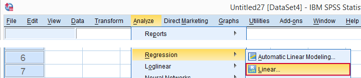
Regression
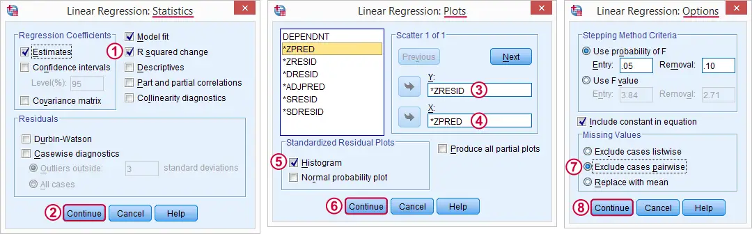
Now that we're sure our data make perfect sense, we're ready for the actual regression analysis. We'll generate the syntax by following the screenshots below.
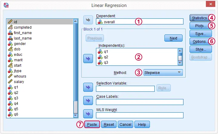
(We'll explain why we choose when discussing our output.)
 -
- Here we select some charts for evaluation the regression assumptions.
 By default, SPSS uses only our 297 complete cases for regression. By choosing this option, our regression will use the correlation matrix we saw earlier and thus use more of our data.
“Stepwise” - What Does That Mean?
When we select the stepwise method, SPSS will include only “significant” predictors in our regression model: although we selected 9 predictors, those that don't contribute uniquely to predicting job satisfaction will not enter our regression equation. In doing so, it iterates through the following steps:
- find the predictor that contributes most to predicting the outcome variable and add it to the regression model if its p-value is below a certain threshold (usually 0.05).
- inspect the p-values of all predictors in the model. Remove predictors from the model if their p-values are above a certain threshold (usually 0.10);
- repeat this process until 1) all “significant” predictors are in the model and 2) no “non significant” predictors are in the model.
Regression Results - Coefficients Table
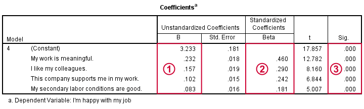
Our coefficients table tells us that SPSS performed 4 steps, adding one predictor in each. We usually report only the final model.
 Our unstandardized coefficients and the constant allow us to predict job satisfaction. Precisely,
Y' = 3.233 + 0.232 * x1 + 0.157 * x2 + 0.102 * x3 + 0.083 * x4
where Y' is predicted job satisfaction, x1 is meaningfulness and so on. This means that respondents who score 1 point higher on meaningfulness will -on average- score 0.23 points higher on job satisfaction.
Our unstandardized coefficients and the constant allow us to predict job satisfaction. Precisely,
Y' = 3.233 + 0.232 * x1 + 0.157 * x2 + 0.102 * x3 + 0.083 * x4
where Y' is predicted job satisfaction, x1 is meaningfulness and so on. This means that respondents who score 1 point higher on meaningfulness will -on average- score 0.23 points higher on job satisfaction.
Importantly, all predictors contribute positively (rather than negatively) to job satisfaction. This makes sense because they are all positive work aspects.
 If our predictors have different scales -not really the case here- we may compare their relative strengths -the beta coefficients- by standardizing them. Like so, we see that meaningfulness (.460) contributes about twice as much as colleagues (.290) or support (.242).
All predictors are highly statistically significant (p = 0.000), which is not surprising considering our large sample size and the stepwise method we used.
Regression Results - Model Summary
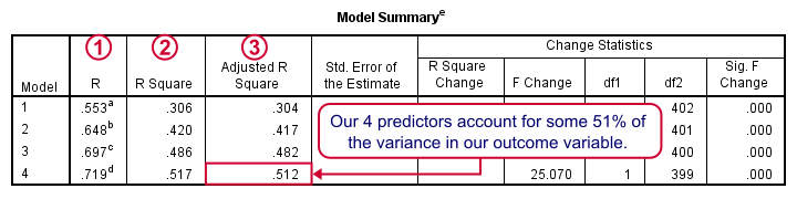
Adding each predictor in our stepwise procedure results in a better predictive accuracy.
R is simply the Pearson correlation between the actual and predicted values for job satisfaction;
R square -the squared correlation- is the proportion of variance in job satisfaction accounted for by the predicted values;
We typically see that our regression equation performs better in the sample on which it's based than in our population. tries to estimate the predictive accuracy in our population and is slightly lower than R square.
We'll probably settle for -and report on- our final model; the coefficients look good it predicts job performance best.
Regression Results - Residual Histogram
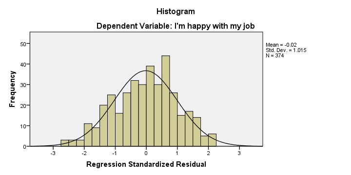
Remember that one of our regression assumptions is that the residuals (prediction errors) are normally distributed. Our histogram suggests that this more or less holds, although it's a little skewed to the left.
Regression Results - Residual Plot
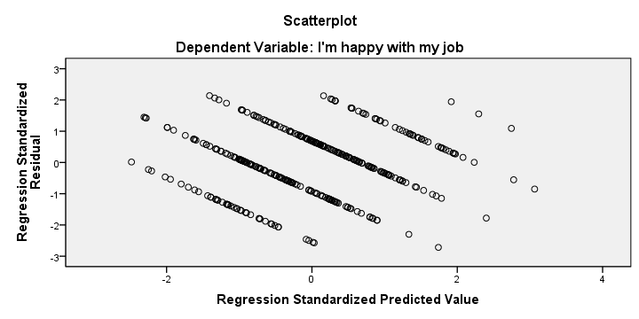
We also created a scatterplot with predicted values on the x-axis and residuals on the y-axis. This chart does not show violations of the independence, homoscedasticity and linearity assumptions but it's not very clear.
We mostly see a striking pattern of descending straight lines. This is because our dependent variable only holds values 1 through 10. Therefore, each predicted value and its residual always add up to 1, 2 and so on. Standardizing both variables may change the scales of our scatterplot but not its shape.
Stepwise Regression - Reporting
There's no full consensus on how to report a stepwise regression analysis.5,7 As a basic guideline, include
- a table with descriptive statistics;
- the correlation matrix of the dependents variable and all (candidate) predictors;
- the model summary table with R square and change in R square for each model;
- the coefficients table with at least the B and β coefficients and their p-values.
Regarding the correlations, we'd like to have statistically significant correlations flagged but we don't need their sample sizes or p-values. Since you can't prevent SPSS from including the latter, try SPSS Correlations in APA Format.
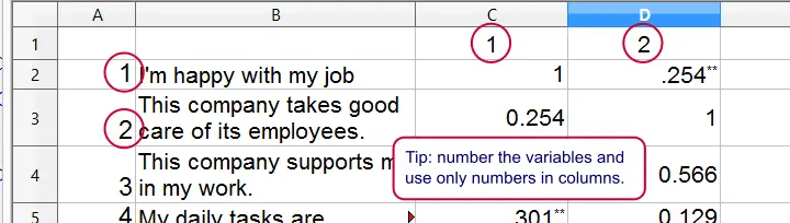
You can further edit the result fast in an OpenOffice or Excel spreadsheet by right clicking the table and selecting
![]() .
.
I guess that's about it. I hope you found this tutorial helpful. Thanks for reading!
References
- Stevens, J. (2002). Applied multivariate statistics for the social sciences. Mahway, NJ: Lawrence Erlbaum Associates.
- Agresti, A. & Franklin, C. (2014). Statistics. The Art & Science of Learning from Data. Essex: Pearson Education Limited.
- Hair, J.F., Black, W.C., Babin, B.J. et al (2006). Multivariate Data Analysis. New Jersey: Pearson Prentice Hall.
- Berry, W.D. (1993). Understanding Regression Assumptions. Newbury Park, CA: Sage.
- Field, A. (2013). Discovering Statistics with IBM SPSS Newbury Park, CA: Sage.
- Howell, D.C. (2002). Statistical Methods for Psychology (5th ed.). Pacific Grove CA: Duxbury.
- Nicol, A.M. & Pexman, P.M. (2010). Presenting Your Findings. A Practical Guide for Creating Tables. Washington: APA.
THIS TUTORIAL HAS 8 COMMENTS:
By Saif khan on November 27th, 2019
Thank you for helpful tutorial,But kindly guide us :How can we address the result of stepwise linear regression in research paper?
By [email protected] on March 7th, 2020
how can i interpret the result of stepwise multiple regression.
By Ruben Geert van den Berg on March 8th, 2020
Hi Jesan!
Very basically, predictors that are excluded from the final model don't add anything to the predictors that are included in the final model when it comes to predicting some outcome variable.
The final model is no different than any other multiple linear regression model. The predicted outcome is a weighted sum of 1+ predictors.
Hope that helps!