SPSS AUTORECODE – Quick Tutorial

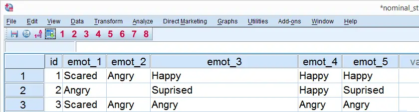
This tutorial explains SPSS’ AUTORECODE command and shows how to use it properly on nominal_strings.sav, a screenshot of which is shown below. We recommend downloading this data file and following along with the steps in this tutorial.

SPSS AUTORECODE - What Is It?

SPSS AUTORECODE creates a new numeric variable from a string variable. The string values are recoded into integer numbers (1, 2, 3 and so on). Each number then receives the string value it represents as a value label.
Regarding our data file, note in variable view that emot_1 through emot_5 are string variables. We'll now AUTORECODE the first one and inspect the result with the syntax below.

SPSS AUTORECODE - Syntax Example 1

Result

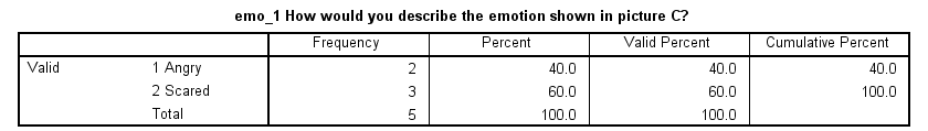
Note in this table that the string values are first sorted alphabetically before they're assigned to numbers 1 and 2.

SPSS AUTORECODE - PRINT Subcommand

Whenever you use AUTORECODE, it's nice to see which string values are converted to which numeric values. We can have SPSS print this coding scheme in the output viewer window by simply adding a PRINT subcommand as shown below.

SPSS AUTORECODE - Syntax Example 2

Result

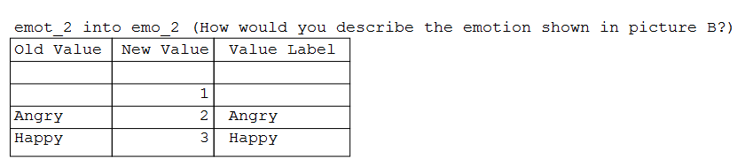
Note that there's something awkward here: it seems as if 2 new values are converted into 3 new values. What's going on is that the new value 1 indicates an empty (zero character) string value. In SPSS logic, that's just another distinct (and valid) string value.
We can see in data view that the second case indeed has an empty string value on emot_2.

SPSS AUTORECODE - BLANKS Subcommand

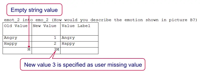
We just saw that AUTORECODE treats empty string values the same as non empty string values. However, we usually see empty string values as missing values and we like to have them recoded last. We can do so by adding a BLANKS subcommand as shown in the syntax below, step 2. Before doing so, we first delete all new variables.

SPSS AUTORECODE - Syntax Example 3

Result

SPSS AUTORECODE - GROUP Subcommand

At this point, note that each AUTORECODE example we ran resulted in a different coding scheme. When we take a close look at our data, however, we see that our string variables mostly contain similar values. This suggests that the same answer categories were used for these 5 questions.
In this common scenario, we usually want to have our new variables consistently coded. That is, we want to have identical value labels over such a set of variables. This is accomplished by adding a GROUP subcommand as shown below.

SPSS AUTORECODE - Syntax Example 4

Result

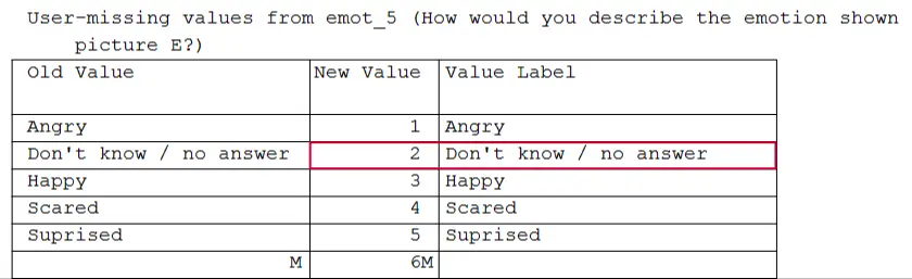
Note that we basically converted the entire data file in one go with our last command. However, there's one thing we don't like: value 2 is used for “Don't know / no answer”. There nothing really wrong with that but it's a bit awkward that this value is among the values used for emotional expressions.
AUTORECODE doesn't have any option for circumventing this but we'll now offer two ways for correcting it.

Option 1: Basic Syntax

One option here is to RECODE 2 into 7 and then adjust the value labels manually. Fortunately, we can do so for all relevant variables simultaneously as shown below.

Option 2: Recode with Value Labels Tool

A much more elegant option for dealing with the “Don't know” values is using our SPSS - Recode with Value Labels Tool. After installing it, it can swap values 2 and 5 together with their value labels by running the syntax below.

SPSS ALTER TYPE – Simple Tutorial

SPSS ALTER TYPE command is mainly used for converting string variables to numeric variables. However, it has other interesting applications as well. This tutorial quickly walks you through those, pointing out some pitfalls, tips and tricks along the way.
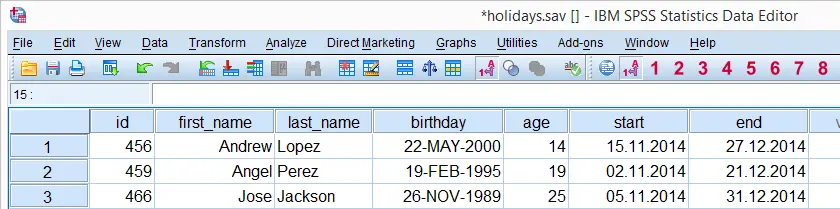
You can follow along by downloading and opening holidays.sav but you do need SPSS version 16 or higher for using ALTER TYPE.

SPSS ALTER TYPE Pitfall

Although ALTER TYPE is a great option for getting many things done fast, it has one major shortcoming: if it fails to convert one or more values, it returns system missing values without throwing any warnings or errors.
If this goes undetected, it may severely damage your data and bias research outcomes. And even if you do notice system missing values resulting from ALTER TYPE, it will be hard to track down what (if anything) went wrong because the original values are overwritten.

Playing it Safe

We propose two basic strategies for playing it safe:

• Always copy your variables before converting them. A great tool for cloning many (or all) variables in your data is freely downloadable from Clone Variables.
• Just run ALTER TYPE on your original variables but check the results for system missings immediately afterwards. If they are present and you don't know why, close your data, rerun you syntax up to the suspicious ALTER TYPE command and inspect what values could cause the problem.

SPSS ALTER TYPE - String to Numeric

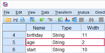
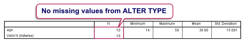
We'd like to know the average age of our participants but we can't calculate it because age is a string variable in our data. The syntax below first copies and converts it to a numeric variable. We can see that no missing values occur in the result by running DESCRIPTIVES; n is equal to the number of cases in our data.

SPSS ALTER TYPE Syntax Example 1

SPSS ALTER TYPE - String to Date

We now turn to birthday. This is a string variable and we wish to convert it to a date variable. Now, SPSS date variables are numeric variables holding numbers of seconds that are displayed as normal dates. They have several display options, a quick overview of which is found under date format. Note that the string values in birthday correspond to what date values look like if their format is set to DATE11. We therefore must specify DATE11 in ALTER TYPE (step 3 below) for converting birthday to a date variable.

SPSS ALTER TYPE Syntax Example 2

SPSS ALTER TYPE - String to Date

Note that start and end are also string variables. Their values look like date values displayed as EDATE10. We'll copy and convert both of them to date variables by the syntax below.

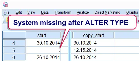
System Missing Values from ALTER TYPE

Note that ALTER TYPE resulted in a system missing value without any warning or error. Fortunately, we copied our variables before converting them and copy_start tells us that the day and month were reversed for one case. Because cases have unique id values, we can easily correct the problem by combining DATE.DMY and IF as shown in the next syntax example.

SPSS ALTER TYPE - Filter

An interesting but little known feature of ALTER TYPE is converting all variables having a given format. We can do so by specifying an input format, which then acts as a filter: ALTER TYPE affects only variables whose formats match this input format. The example below first addresses all variables but only converts those having an EDATE format.

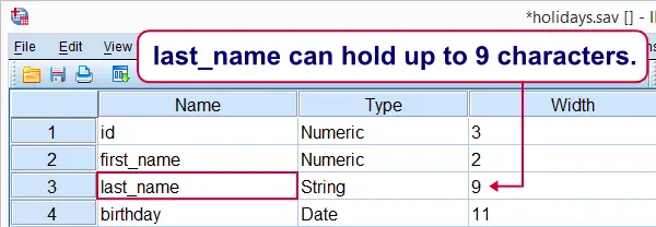
SPSS ALTER TYPE - Change String Lengths

ALTER TYPE can change the lengths of string variables. For example, the last respondent in our data got married and changed her last name to “Hernandez-Garcia”. We can't readily correct this: as we can see in variable view, last_name has an A9 format and can thus hold up to 9 characters.

The syntax below solves this by increasing its length with ALTER TYPE.

Value Labels of Numeric Variable to String Variable

Note that first_name is a numeric variable in our data. We can change it to a string variable with ALTER TYPE but this will convert the values (1 through 10) instead of the last names, which are in the value labels. The solution is using VALUELABEL but the entire process requires some manual steps outlined in the syntax below.

SPSS ALTER TYPE - Minimize String Lengths

A nice ALTER TYPE trick is minimizing the lengths of all string variables in the data. We can do so by setting all A formats to AMIN: a special ALTER TYPE keyword denoting the minimum length for each string variable.
In the previous examples, we guessed that 30 characters would be enough for first_name and last_name. These lengths are actually longer than necessary, causing the size of the data file to increase. We can easily minimize all string lengths by using the aforementioned filter feature: alter type all(a = amin).

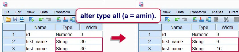
As we see from the result, the minimal required lengths for first_name and last_name are 9 and 16.

SPSS ADD FILES Command

Summary

ADD FILES is an SPSS command that's mainly used for merging data sources holding similar variables but different cases. (For the same cases but different variables, see MATCH FILES.) A second use is for reordering and/or dropping variables in a single dataset. SPSS Add Files Matches Data Sources on Variable Names

SPSS Add Files - Basic Usage

The ADD FILES command illustrated in the screenshot above results from running the syntax below.

SPSS Add Files Syntax Example

SPSS Add Files Rules

• Up to 50 datasets or data files can be merged with a single ADD FILES command.
• ADD FILES can also be used for reordering and/or dropping variables in a single dataset. This is done by using the KEEP or DROP subcommand. How it works is explained in MATCH FILES.

SPSS Add Files Pitfalls

• If a variable has inconsistent dictionary information across data sources, you may end up with nonsensical data. This is explained in SPSS Recode - Cautionary Note. For a tool that detects dictionary inconsistencies over files, see Compare Dictionaries over Files Before Merging.
• If there are string variables present, they should have the same lengths across all data sources. Adjust String Lengths before Merging Files shows how to do this automatically using Python.
• Especially with many data files, you may want to add the file names as a new variable to the files. Like so, you can easily see the source of each case in the merged data. See Add Filenames to Files Before Merging.
• An alternative for adding the data sources to the merged result is using the IN subcommand as in add files file d1 /in = d1 / file d2 /in = d2.
• If you want to merge a lot of files, you can have Python do it for you. This is demonstrated in !!0250.

SPSS AGGREGATE Command

Aggregate is an SPSS command for creating variables holding statistics over cases. This tutorials briefly demonstrates the most common scenarios and points out some best practices.

SPSS Aggregate Command

The SPSS AGGREGATE command typically works like so:

• One or more BREAK variables can be specified.In SPSS versions 15 and below, specifying at least one BREAK variable is mandatory. If you want statistics over all cases, use compute constant = 0. and use constant as the BREAK variable.
• All cases with the same value(s) on the break variable(s) are referred to as a break group
• Each break group will become a single case in the aggregated data (unless MODE = ADDVARIABLES is used).
• This new case has summary statistics over the original cases as new variables. Available statistics include the frequency, mean, maximum and many others. Consult the command syntax reference for a complete overview.
• The result of AGGREGATE may be the active dataset, a new dataset or a new data file. (This last option is not available for MODE = ADDVARIABLES.) A new Dataset must first be declared before it can be specified in AGGREGATE.
• For a very basic demonstration, run the syntax below.

SPSS Aggregate Syntax Example

MODE = ADDVARIABLES

SPSS Aggregate - Mode = Addvariables

Except for SPSS versions 12 and below, summary statistics of break groups can be appended to a Dataset without actually aggregating it. The syntax below demonstrates this.

SPSS Aggregate Syntax Example

Statistics over Multiple Variables

Summary statistics can be rendered over multiple variables in one go. The TO and ALL keywords can conveniently shorten the list of variables as shown in the syntax below.

Multiple Statistics

Different summary statistics (over the same or different variables) can be specified in a single command. This is demonstrated below (uses test data from previous example).

Final Note

Lots of different things can be done with the AGGREGATE command. This tutorial aimed at illustrating the most common scenarios found in practice. It is by no means intended as an exhaustive overview of all options.