SPSS RECODE – Simple Tutorial

Introduction

SPSS RECODE replaces data values with different values. It comes in handy for merging categories, dichotomizing continuous variables and some other tasks. This tutorial walks you through its main options, best practices and pitfalls.

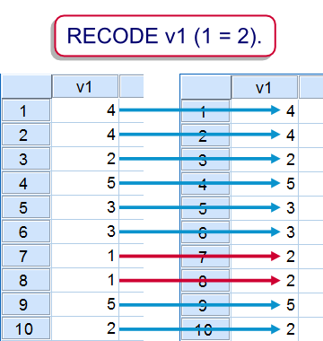SPSS Recode Example 1

For quickly getting very proficient with RECODE it's recommended you follow along with the examples. You'll soon notice that recoding from syntax is very simple and way, way faster than from the GUI. All examples use supermarket.sav.

1. Merge Categories of One Variable

In this example we'll merge categories 1 and 2 of a variable v1. We'll do this by changing all values of 1 into 2. This is as simple as recode v1 (1 = 2).The screenshot illustrates the effect. All values that are not 1 are left unaltered. We'll run FREQUENCIES right before and after recoding so we can check the results.

SPSS Recode Syntax Example 1

Note that after recoding the value labels are no longer correct.For more on this, see SPSS Recode - Cautionary Note. We therefore adjust the value label for 2 and remove the label for 1.

2. Dichotomize Multiple Variables

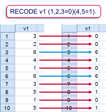SPSS Recode Example 2

We'll dichotomize variables v4 to v6 by changing values 1, 2 and 3 into 0 and values 4 and 5 into 1 as implied byrecode v4 to v6 (1,2,3 = 0)(4,5 = 1).Value 6 is is left unaltered. After recoding we must respecify the value labels for all three variables. The reason why we need two quotes in don''t know is explained in Escape Sequence (General Concept).

SPSS Recode Syntax Example 2

3. Merge Categories into New Variable

In the previous examples the original values were overwritten by the recoded values. An alternative is creating a new variable holding the recoded values. This is done by using the INTO keyword like sorecode v2 (1=2) into rec_v2.However, this doesn't tell which values rec_v2 should hold if v2 is not 1, resulting in lots of system missing values. Here we can use ELSE, which means “all values that were not previously addressed”. For copying them from v2 into rec_v2 we'll use (ELSE = COPY).

SPSS Recode Syntax Example 3

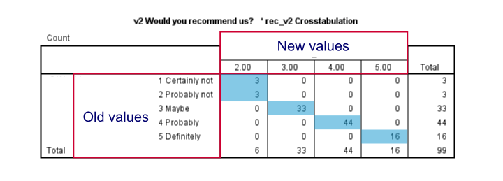A crosstab confirms that categories 1 and 2 have been merged into 2.

This example shows some disadvantages of recoding into new variables. First, note that the new variables don't have any dictionary information at all.
Second, the new variables are appended to the end of the active dataset. Therefore, you can't address a range of original and recoded variables by using the TO ALL keywords. However, an easy way to reorder is using MATCH FILES.

4. Dichotomize Multiple Variables into New Variables

Recoding several variables into several new variables is straightforward: simply fill in multiple input variable names after RECODE and multiple output variable names after INTO. Just make sure that the number of input variables matches the number of output variables.
This example uses LO THRU 3 which means “the lowest value through 3”. In a similar vein, HI can be used for the highest value.
Optionally, users who have the SPSS Python Essentials installed can generate the crosstabs in a loop as shown in step 3B.

SPSS Recode Syntax Example 4

5. Recode Continuous into Discrete Variable

Values are recoded only once by RECODE. The old and new value pairs are read from left to right and an old value that's already been addressed will be ignored if it's addressed again. This is also the reason that there's no point in specifying any old values after the ELSE keyword.
This feature is sometimes used when discretizing continuous variables: you can use LO (the lowest value that hasn't been previously addressed) as the lower boundary for each category. The syntax below looks a bit awkward but is not unusual. As demonstrated, a descriptives by category table is a nice way to inspect these results. Finally, note that RANK offers an alternative for discretizing variables.

SPSS Recode Syntax Example 5

6. Clone a Variable

A disadvantage of recoding into new variables is they don't have any dictionary information by default. However, we can clone a variable with its dictionary information by combining RECODE with APPLY DICTIONARY. This is basically what our SPSS Clone Variables Tool does for many variables at once.The tool also checks whether input variables are string variables. If so, it automatically declares the new string variables with the correct lengths that are needed for recoding into.
After cloning, we can safely recode into the same variables, leaving the variable order intact and minimizing the need for dictionary modifications after recoding. In case of doubt we can always check the recoded variable against its clone and if necessary delete it and start over from a new clone.

SPSS Recode Syntax Example 6

7. Recode String to Numeric Variable

In some cases you may want to recode a string variable into a numeric one. This holds especially when you want to do calculations on ordinal variables under the Assumption of Equal Intervals.Note that we can't use AUTORECODE here because we don't want our values to follow the alphabetical order of our string values.
Keep in mind that you can RECODE and apply value labels to many variables at once. Unfortunately, copying the variable labels from the old to the new variables requires some more work but this can be automated with Python if desired.

SPSS Recode Syntax Example 7

Final Notes

This tutorial didn't cover some more exotic RECODE options. The reason is that we rarely see these in practice and we didn't want to go into detail any further than we already did. Some more options than described here are covered by the command syntax reference.

SPSS RANGE Function – Quick Tutorial

COMPUTE v2 = RANGE(V1,2,4).

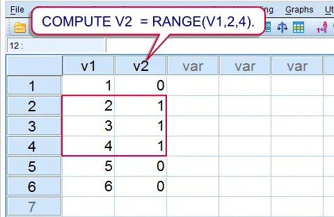SPSS RANGE Function Result

Summary

SPSS’ RANGE function is used to evaluate whether or not values are within a given range. Test values equal to the lower or upper boundary are also within the given range. Run the syntax below for a quick demonstration.

SPSS Range Syntax Example

Notes

RANGE takes three arguments. So in RANGE(A,B,C)

• A refers to the test value;
• B refers to the lower boundary;
• C refers to the upper boundary;
• A, B and C can all be values within variables or constants (over cases). The most common scenario, however, is that A is a variable and B and C constants.

RANGE may return three values:

• 1 (or “True”) if the test value is within the range;
• 0 (or “False”) if the test value is not within the range;
• A system missing value if the range can't be evaluated due to missing values.

SPSS Range with Dates and Times

SPSS RANGE can be readily used with date variables and time variables. It should be kept in mind that SPSS dates and times are expressed in numbers of seconds. This implies that you should convert “normal” date and time values into numbers of seconds too. This can be done with the DATE.DMY and TIME.HMS functions as shown in the syntax below.Minutes and seconds default to zero in TIME.HMS. That is, TIME.HMS(18,0,0) may be shortened to TIME.HMS(18).

SPSS Range Syntax Example

SPSS Range with Strings

Technically, you can use RANGE for string values too. SPSS basically uses an alphabetical order to determine whether string values are in a given range or not. This can be seen by running SORT CASES as in the syntax example below.

SPSS Range Syntax Example

SPSS RANK Command

Summary

SPSS RANK can be used to create a variable holding the rank numbers of the values of some other variable. RANK is also used for discretizing continuous variables into ntile groups. This tutorial walks you through the main options along with some real world examples.

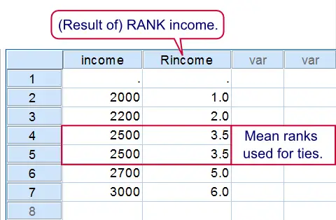Result of first RANK syntax example

1. SPSS Rank Basic Example

Running the syntax below first creates a mini dataset and then ranks income (the result is shown in the screenshot). The default name for the new variable is R + the old variable name, resulting in Rincome. Note that a system missing value does not get any rank number. A value occurring more than once is referred to as a tie. By default, mean rank numbers are assigned to ties.

SPSS Rank Syntax Example 1

2. Creating Ntiles

The following examples will all use employees.sav. The syntax below shows how to create four age groups of equal sizes by using RANK. (If the sample size is not divisible by the number of groups or ties are present, SPSS will attempt to make the group sizes as equal as possible.) In first instance the new variable is called Ndate_of where the N denotes Ntiles.SPSS uses a maximum of 8 letters for new variable names created by RANK. This is why we don't get Ndate_of_birth (as we may have expected). In step 4, we'll use MEANS for inspecting the result.

SPSS Rank Syntax Example 2

3. Rank Within Groups

Thus far we used RANK with regard to the entire sample. However, we may also RANK within groups defined by one or more variables. Like so, the syntax below creates median age groups within each gender separately. When these are combined with gender we'll get four groups indicating the 50% youngest women, the 50% oldest women and so on. Note that we undo all changes made to the data thus far by simply reopening it.

SPSS Rank Syntax Example 3

4. Rank Into

In the second example we used a basic RANK command and then used RENAME for changing the name of the new variable. Alternatively, we can specify a new variable name within RANK itself by using the INTO keyword as demonstrated by the syntax below.

SPSS Rank Syntax Example 4

5. Rank Multiple Variables

If you'd like to RANK multiple variables, you can do so in a single command. Like so, the final example below create median groups for date_of_birth, experience_years and monthly_income.

SPSS Rank Syntax Example 5

6. Ranking Descendingly

If you paid close attention, you may have noticed something awkward in the previous example: for dic_experience and dic_income a higher value indicates more experience/income. However, for dic_age the reverse holds. This is because we used date_of_birth which is related inversely to age.
One solution is to first compute raw age (also see How to Compute Age in SPSS?) and use that instead. However, an easier way out is to RANK (only) date_of_birth descendingly. Simply replacing RANK date_of_birth by RANK date_of_birth (D) in the last syntax does the trick here.

Final Note

• Note that ranking into ntiles is quite similar to RECODE. However, with RANK the values that separate ntile groups depend on the data whereas with RECODE the group sizes depend on the data.