Kendall’s Tau – Simple Introduction

Kendall’s Tau is a number between -1 and +1
that indicates to what extent 2 variables are monotonously related.

• Kendall’s Tau - Formulas
• Kendall’s Tau - Exact Significance
• Kendall’s Tau - Confidence Intervals
• Kendall’s Tau versus Spearman Correlation
• Kendall’s Tau - Interpretation

Kendall’s Tau - What is It?

Kendall’s Tau is a correlation suitable for quantitative and ordinal variables. It indicates how strongly 2 variables are monotonously related: to which extent are high values on variable x are associated with
either high or low values on variable y? Like so, Kendall’s Tau serves the exact same purpose as the Spearman rank correlation. The reasoning behind the 2 measures, however, is different. Let's take a look at the example data shown below.

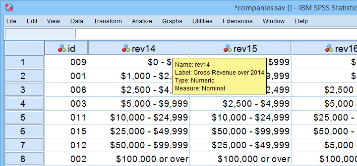
These data show yearly revenues over the years 2014 through 2018 for several companies. We'd like to know to what extent companies that did well in 2014 also did well in 2015. Note that we only have revenue categories and these are ordinal variables: we can rank them but we can't compute means, standard deviations or correlations over them.

Kendall’s Tau - Intersections Method

If we rank both years, we can inspect to what extent these ranks are different. A first step is to connect the 2014 and the 2015 ranks with lines as shown below.

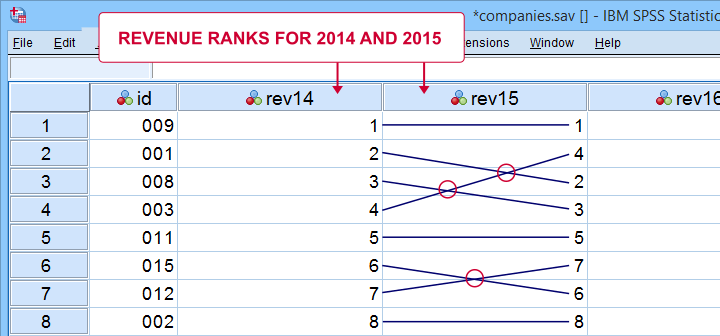
Our connection lines show 3 intersections. These are caused by the 2014 and 2015 rankings being slightly different. Note that the more the ranks differ, the more intersections we see:

• if 2 rankings are identical, we have zero intersections and
  
• if 2 rankings are exactly opposite, the number of intersections is

$$0.5\cdot n(n - 1)$$
This is the maximum number of intersections for \(n\) observations. Dividing the actual number of intersections by the maximum number of intersections is the basis for Kendall’s tau, denoted by \(\tau\) below.

$$\tau = 1 - \frac{2\cdot I}{0.5\cdot n(n - 1)}$$
where \(I\) is the number of intersections. For our example data with 3 intersections and 8 observations, this results in

$$\tau = 1 - \frac{2\cdot 3}{0.5\cdot 8(8 - 1)} =$$
$$\tau = 1 - \frac{6}{28} \approx 0.786$$

Since \(\tau\) runs from -1 to +1, \(\tau\) = 0.786 indicates a strong positive relation: higher revenue ranks in 2014 are associated with higher ranks in 2015.

Kendall’s Tau - Concordance Method

A second method to find Kendall’s Tau is to inspect all unique pairs of observations. We did so in this Googlesheet shown below.

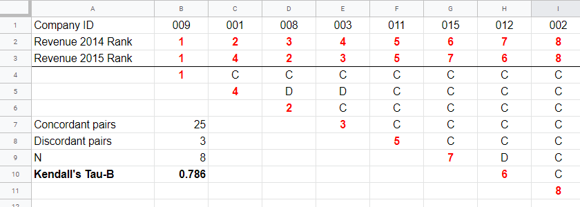
Starting at row 4, each 2015 rank is compared to all 2014 ranks to its right. If these are higher, we have concordant pairs of observations denoted by C. These indicate a positive relation.

However, 2015 ranks having larger 2014 ranks to their right indicate discordant pairs denoted by D. For instance, cell D5 is discordant because the 2014 rank (3) is smaller than the 2015 rank of 4. Discordant pairs indicate a negative relation.

Finally, Kendall’s Tau can be computed from the numbers of concordant and discordant pairs with $$\tau = \frac{n_c - n_d}{0.5\cdot n(n - 1)}$$

for our example with 3 discordant and 25 concordant pairs in 8 observations, this results in $$\tau = \frac{25 - 3}{0.5\cdot 8(8 - 1)} = $$
$$\tau = \frac{22}{28} \approx 0.786.$$
Note that C and D add up to the number of unique pairs of observations, \(0.5\cdot n(n - 1)\) which results 28 in our example. Keeping this in mind, you may see that

• \(\tau\) = -1 if all pairs are discordant;
• \(\tau\) = 0 if the numbers of concordant and discordant pairs are equal and
• \(\tau\) = 1 if all pairs are concordant.

Kendall’s Tau-B & Tau-C

Our first method for computing Kendall’s Tau only works if each company falls into a different revenue category. This holds for the 2014 and 2015 data. For 2017 and 2018, however, some companies fall into the same revenue categories. These variables are said to contain ties. Two modified formulas are used for this scenario:

• Kendall’s tau-b corrects for ties and
• Kendall’s tau-c ignores ties.

Simply “Kendall’s Tau” usually refers Kendall’s Tau-b. We won't discuss Kendall’s Tau-c as it's not often used anymore. In the absence of ties, both formulas yield identical results.

Kendall’s Tau - Formulas

So how could we deal with ties? First off, mean ranks are assigned to tied observations as in this Googlesheet shown below: companies 009 and 001 share the two lowest 2016 ranks so they are both ranked the mean of ranks 1 and 2, resulting in 1.5.

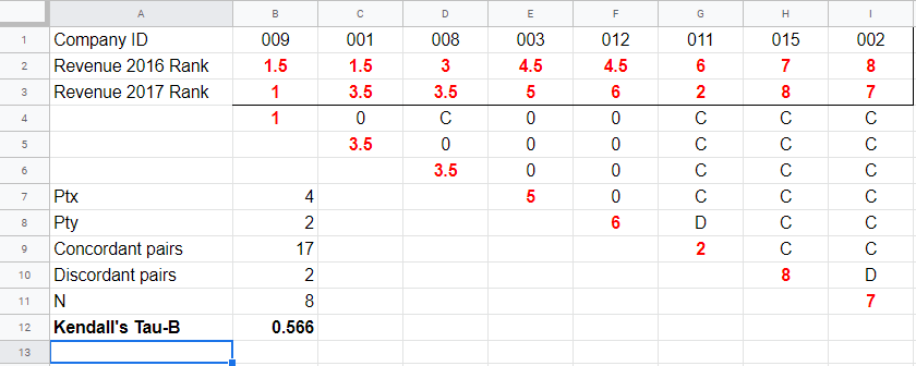
Second, pairs associated with tied 2016 observations are neither concordant nor discordant. Such pairs (columns B,C and E,F) receive a 0 rather than a C or a D. Third, 2017 ranks that have a 2017 tie to their right are also assigned 0. Like so, the 28 pairs in the example above result in

• 17 concordant pairs (C),
• 2 discordant pairs (D) and
• 9 inconclusive pairs (0).

For computing \(\tau_b\), ties on either variable result in a penalty computed as $$Pt = \Sigma{(t_i^2 - t_i)}$$
where \(t_i\) denotes the length of the \(i\)th tie for either variable. The 2016 ranks have 2 ties -both of length 2- resulting in $$Pt_{2016} = (2^2 - 2) + (2^2 - 2) = 4$$
Similarly, $$Pt_{2017} = (2^2 - 2) = 2$$

Finally, \(\tau_b\) is computed with $$\tau_b = \frac{2\cdot (C - D)}{\sqrt{n(n - 1) - Pt_x}\sqrt{n(n - 1) - Pt_y}}$$

For our example, this results in $$\tau_b = \frac{2\cdot (17 - 2)}{\sqrt{8(8 - 1) - 4}\sqrt{8(8 - 1) - 2}} =$$
$$\tau_b = \frac{30}{\sqrt{52}\sqrt{54}} \approx 0.566$$

Kendall’s Tau - Exact Significance

For small sample sizes of N ≤ 10, the exact significance level for \(\tau_b\) can be computed with a permutation test. The table below gives critical values for α = 0.05 and α = 0.01.

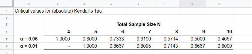
Our example calculation without ties resulted in \(\tau_b\) = 0.786 for 8 observations. Since \(|\tau_b|\) > 0.7143, p < 0.01: we reject the null hypothesis that \(\tau_b\) = 0 in the entire population. Basic conclusion: revenues over 2014 and 2015 are likely to have a positive monotonous relation in the entire population of companies.

The second example (with ties) resulted in \(\tau_b\) = 0.566 for 8 observations. Since \(|\tau_b|\) < 0.5714, p > 0.05. We retain the null hypothesis: our sample outcome is not unlikely if revenues over 2016 and 2017 are not monotonously related in the entire population.

Kendall’s Tau-B - Asymptotic Significance

For sample sizes of N > 10, $$z = \frac{3\tau_b\sqrt{n(n - 1)}}{\sqrt{2(2n + 5)}}$$

roughly follows a standard normal distribution. For example, if \(\tau_b\) = 0.500 based on N = 12 observations, $$z = \frac{3\cdot 0.500 \sqrt{12(11)}}{\sqrt{2(24 + 5)}} \approx 2.263$$

We can easily look up that \(p(|z| \gt 2.263) \approx 0.024\): we reject the null hypothesis that \(\tau_b\) = 0 in the population at α = 0.05 but not at α = 0.01.

Kendall’s Tau - Confidence Intervals

Confidence intervals for \(\tau_b\) are easily obtained from JASP. The screenshot below shows an output example.

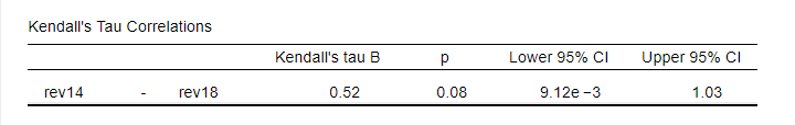
We presume that these confidence intervals require sample sizes of N > 10 but we couldn't find any reference on this.

Kendall’s Tau versus Spearman Correlation

Kendall’s Tau serves the exact same purpose as the Spearman rank correlation: both indicate to which extent 2 ordinal or quantitative variables are monotonously related. So which is better? Some general guidelines are that

1. the statistical properties -sampling distribution and standard error- are better known for Kendall’s Tau than for Spearman-correlations. Kendall’s Tau also converges to a normal distribution faster (that is, for smaller sample sizes). The consequence is that significance levels and confidence intervals for Kendall’s Tau tend to be more reliable than for Spearman correlations.
2. absolute values for Kendall’s Tau tend to be smaller than for Spearman correlations: when both are calculated on the same data, we typically see something like \(|\tau_b| \approx 0.7\cdot |R_s|\).
3. Kendall’s Tau typically has smaller standard errors than Spearman correlations. Combined with the previous point, the significance levels for Kendall’s Tau tend to be roughly equal to those for Spearman correlations.

In order to illustrate point 2, we computed Kendall’s Tau and Spearman correlations on 8 simulated variables, v1 through v8. The colors shown below are linearly related to the absolute values.

For basically all cells, the second line (Spearman correlation) is darker, indicating a larger absolute value. Also, \(|\tau_b| \approx 0.7\cdot |R_s|\) seems a rough but reasonable rule of thumb for most cells.

The significance levels for the same variables are shown below.

These colors show no clear pattern: sometimes Kendall’s Tau is “more significant” than Spearman’s rho and sometimes the reverse is true. Also note that the significance levels tend to be more similar than the actual correlations. Sadly, the positive skewness of these p-values results in limited dispersion among the colors.

Kendall’s Tau - Interpretation

• \(\tau_b\) = -1 indicates a perfect negative monotonous relation among 2 variables: a lower score on variable A is always associated with a higher score on variable B;
• \(\tau_b\) = 0 indicates no monotonous relation at all;
• \(\tau_b\) = 1 indicates a perfect positive monotonous relation: a lower score on variable A is always associated with a lower score on variable B.

The values of -1 and +1 can only be attained if both variables have equal numbers of distinct ranks, resulting in a square contingency table.

Furthermore, if 2 variables are independent, \(\tau_b\) = 0 but the reverse does not always hold: a curvilinear or other non monotonous relation may still exist.

We didn't find any rules of thumb for interpreting \(\tau_b\) as an effect size so we'll propose some:

• \(|\tau_b|\) = 0.07 indicates a weak association;
• \(|\tau_b|\) = 0.21 indicates a medium association;
• \(|\tau_b|\) = 0.35 indicates a strong association.

Kendall’s Tau-B in SPSS

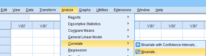
The simplest option for obtaining Kendall’s Tau from SPSS is from the correlations dialog as shown below.

Alternatively (and faster), use simplified syntax such as

Thanks for reading!

Kendall’s Tau in SPSS – 2 Easy Options

• Example Data File
• Kendall’s Tau-B from Correlations Menu
• Kendall’s Tau-B & Tau-C from Crosstabs
• Wrong Significance Levels for Small Samples

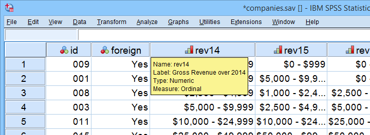
Example Data File

A survey among company owners included the question “what was your yearly revenue?” for several years. The data -partly shown below- are in companies.sav.

Our main research question for today is to what extent are yearly revenues interrelated? Are the best performing companies in 2014 the same as in 2015 and other years? Or do we have entirely different “winners” from year to year?
If we had the exact yearly revenues, we could have gone for Pearson correlation among years and perhaps proceed with some regression analyses.
However, our data contain only revenue categories and these are ordinal variables. This leaves us with 2 options: we can inspect either

• Spearman rank correlations or
• Kendall’s tau.

Although both statistics are appropriate, we'll go for Kendall’s tau: its standard error and sampling distribution are better known and the latter converges to a normal distribution faster.

Filtering Out Domestic Companies.

We'll restrict our analyses to foreign companies by using a FILTER. Since this variable only contains 1 (foreign) and 0 (domestic), a single line of syntax is all we need.

Kendall’s Tau-B from Correlations Menu

The easiest option for Kendalls tau-b is the correlations menu as shown below.

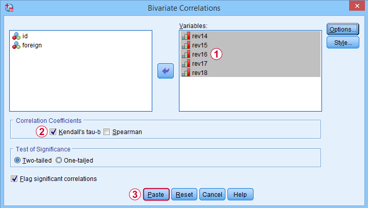
Move all relevant variables into the variables box,
select Kendall’s tau-b and
clicking Paste results in the syntax below. Let's run it.

Result

SPSS creates a full correlation matrix, part of which is shown below.

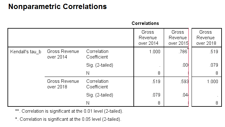
Note that most Kendall correlations are (very) high. This means that companies that perform well in one year
typically perform well in other years too. Despite our minimal sample size, many Kendall correlations are statistically significant. The p-values are identical to those obtained from rerunning the analysis in JASP.

Kendall’s Tau-B and Tau-C from Crosstabs

An alternative method for obtaining Kendalls tau from SPSS is from CROSSTABS. We only recommend this if

• you're going to run CROSSTABS anyway -probably for obtaining chi-square tests;
• you need Kendall’s tau-c instead of tau-b;

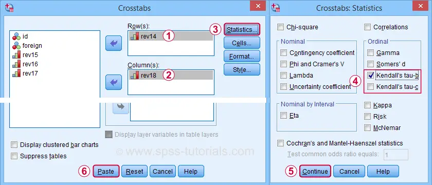
In such cases, you could access the Crosstabs dialog as shown below.

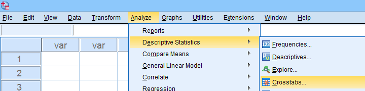
A lot of useful association measures -including Cramér’s V and eta squared- are found under Statistics.
Select either Kendall’s tau-b and/or tau-c -although the latter is rarely reported.
Clicking Paste results in the syntax below.

Wrong Significance Levels for Small Samples

Although Kendall’s tau obtained from CROSSTABS is correct, some of the other results are awkward at best.

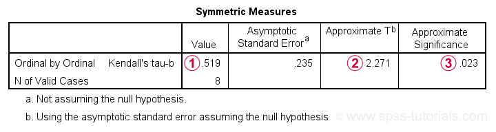
Kendall’s tau-b is identical to that obtained from the correlations dialog;
The Approximate T is a z-value rather than a t-value: it's approximately normally distributed but only for reasonable sample sizes. It cannot be used for the small sample size used in this example.
As a result, the Approximate Significance is wildly off: SPSS comes up with p = 0.079 for the exact same data when using the correlations dialog. This is the exact p-value that should be used for small sample sizes.

“Officially”, the approximate significance may be used for N > 10 but perhaps it's better avoided if N < 20 or so. In such cases, it may be wiser to run Kendall’s tau from the Correlations dialog than from Crosstabs.

Thanks for reading.