• Multiple Regression - Example
• Data Checks and Descriptive Statistics
• SPSS Regression Dialogs
• SPSS Multiple Regression Output
• Multiple Regression Assumptions
• APA Reporting Multiple Regression

Multiple Regression - Example

A scientist wants to know if and how health care costs can be predicted from several patient characteristics. All data are in health-costs.sav as shown below.

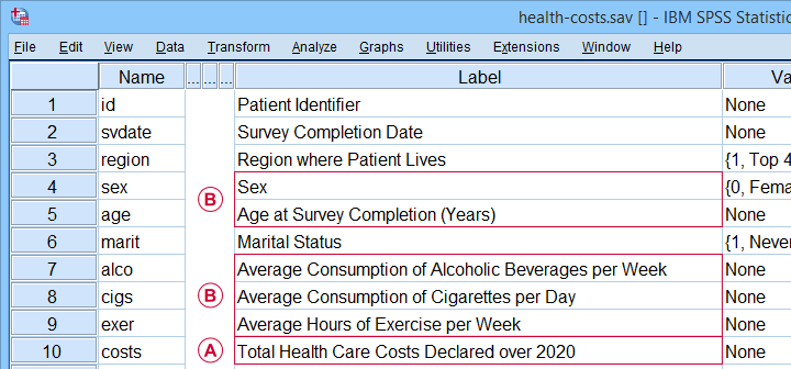
The dependent variable is health care costs (in US dollars) declared over 2020 or “costs” for short.
The independent variables are sex, age, drinking, smoking and exercise.

Our scientist thinks that each independent variable has a linear relation with health care costs. He therefore decides to fit a multiple linear regression model. The final model will predict costs from all independent variables simultaneously.

Data Checks and Descriptive Statistics

Before running multiple regression, first make sure that

1. the dependent variable is quantitative;
2. each independent variable is quantitative or dichotomous;
3. you have sufficient sample size.

A visual inspection of our data shows that requirements 1 and 2 are met: sex is a dichotomous variable and all other relevant variables are quantitative. Regarding sample size, a general rule of thumb is that you want to use at least 15 independent observations
for each independent variable you'll include. In our example, we'll use 5 independent variables so we need a sample size of at least N = (5 · 15 =) 75 cases. Our data contain 525 cases so this seems fine.

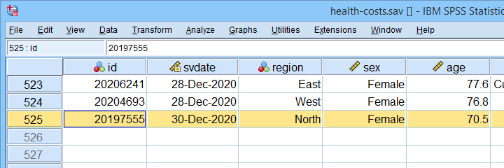Note that we've N = 525 independent observations in our example data.

Keep in mind, however, that we may not be able to use all N = 525 cases if there's any missing values in our variables.

Let's now proceed with some quick data checks. I strongly encourage you to at least

1. run basic histograms over all variables. Check if their frequency distributions look plausible. Are there any outliers? Should you specify any missing values?
2. inspect a scatterplot for each independent variable (x-axis) versus the dependent variable (y-axis).A handy tool for doing just that is downloadable from SPSS - Create All Scatterplots Tool. Do you see any curvilinear relations or anything unusual?
3. run descriptive statistics over all variables. Inspect if any variables have any missing values and -if so- how many.
4. inspect the Pearson correlations among all variables. Absolute correlations exceeding 0.8 or so may later cause complications (known as multicollinearity) for the actual regression analysis.

The APA recommends you combine and report these last two tables as shown below.

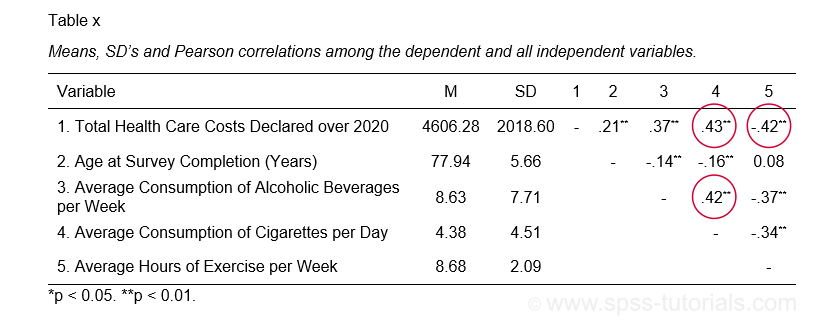APA recommended table for reporting correlations and descriptive statistics
as part of multiple regression results

These data checks show that our example data look perfectly fine: all charts are plausible, there's no missing values and none of the correlations exceed 0.43. Let's now proceed with the actual regression analysis.

SPSS Regression Dialogs

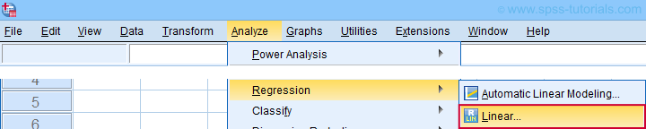
We'll first navigate to Analyze Regression Linear as shown below.

Next, we fill out the main dialog and subdialogs as shown below.

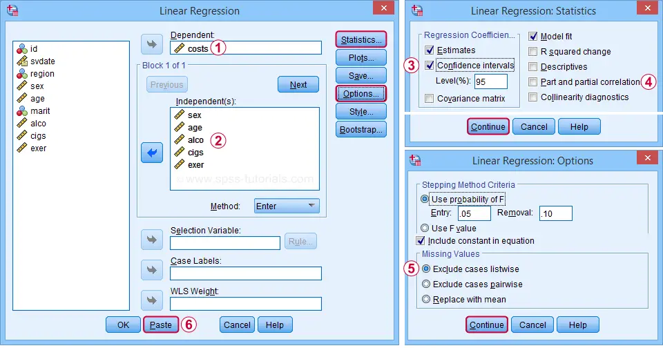
We'll select 95% confidence intervals for our b-coefficients.
Some analysts report squared semipartial (or “part”) correlations as effect size measures for individual predictors. But for now, let's skip them.
By selecting “Exclude cases listwise”, our regression analysis uses only cases without any missing values on any of our regression variables. That's fine for our example data but this may be a bad idea for other data files.
Clicking Paste results in the syntax below. Let's run it.

SPSS Multiple Regression Syntax I

SPSS Multiple Regression Output

The first table we inspect is the Coefficients table shown below.

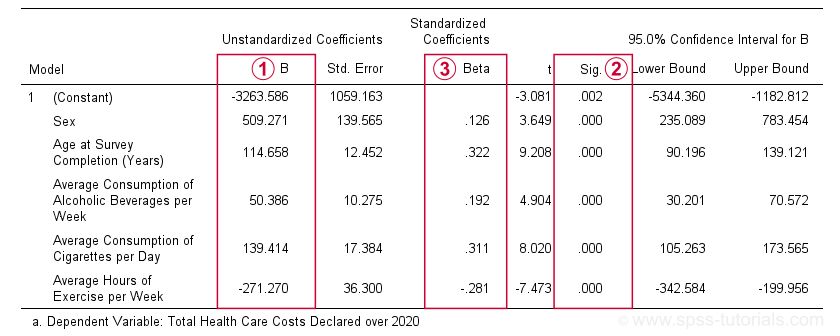
The b-coefficients dictate our regression model:

$$Costs' = -3263.6 + 509.3 \cdot Sex + 114.7 \cdot Age + 50.4 \cdot Alcohol\\ + 139.4 \cdot Cigarettes - 271.3 \cdot Exericse$$

where \(Costs'\) denotes predicted yearly health care costs in dollars.

Each b-coefficient indicates the average increase in costs associated with a 1-unit increase in a predictor. For example, a 1-year increase in age results in an average $114.7 increase in costs. Or a 1 hour increase in exercise per week is associated with a -$271.3 increase (that is, a $271.3 decrease) in yearly health costs.

Now, let's talk about sex: a 1-unit increase in sex results in an average $509.3 increase in costs. For understanding what this means, please note that sex is coded 0 (female) and 1 (male) in our example data. So for this variable, the only possible 1-unit increase is from female (0) to male (1). Therefore, B = $509.3 simply means that the average yearly costs for males
are $509.3 higher than for females (everything else equal, that is). This hopefully clarifies how dichotomous variables can be used in multiple regression. We'll expand on this idea when we'll cover dummy variables in a later tutorial.

The “Sig.” column in our coefficients table contains the (2-tailed) p-value for each b-coefficient. As a general guideline, a b-coefficient is statistically significant if its “Sig.” or p < 0.05. Therefore, all b-coefficients in our table are highly statistically significant. Precisely, a p-value of 0.000 means that if some b-coefficient is zero in the population (the null hypothesis), then there's a 0.000 probability of finding the observed sample b-coefficient or a more extreme one. We then conclude that the population b-coefficient probably wasn't zero after all.

Now, our b-coefficients don't tell us the relative strengths of our predictors. This is because these have different scales: is a cigarette per day more or less than an alcoholic beverage per week? One way to deal with this, is to compare the standardized regression coefficients or beta coefficients, often denoted as β (the Greek letter “beta”).In statistics, β also refers to the probability of committing a type II error in hypothesis testing. This is why (1 - β) denotes power but that's a completely different topic than regression coefficients.

Beta coefficients (standardized regression coefficients) are useful for comparing the relative strengths of our predictors. Like so, the 3 strongest predictors in our coefficients table are:

• age (β = 0.322);
• cigarette consumption (β = 0.311);
• exercise (β = -0.281).

Beta coefficients are obtained by standardizing all regression variables into z-scores before computing b-coefficients. Standardizing variables applies a similar standard (or scale) to them: the resulting z-scores always have mean of 0 and a standard deviation of 1.
This holds regardless whether they're computed over years, cigarettes or alcoholic beverages. So that's why b-coefficients computed over standardized variables -beta coefficients- are comparable within and between regression models.

Right, so our b-coefficients make up our multiple regression model. This tells us how to predict yearly health care costs. What we don't know, however, is precisely how well does our model predict these costs? We'll find the answer in the model summary table discussed below.

SPSS Regression Output II - Model Summary & ANOVA

The figure below shows the model summary and the ANOVA tables in the regression output.

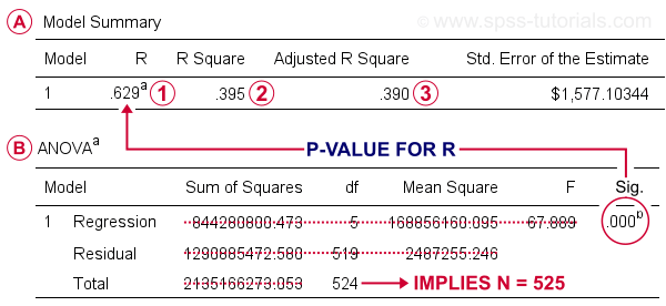
R denotes the multiple correlation coefficient. This is simply the Pearson correlation between the actual scores and those predicted by our regression model.
R-square or R² is simply the squared multiple correlation. It is also the proportion of variance in the dependent variable accounted for by the entire regression model.
R-square computed on sample data tends to overestimate R-square for the entire population. We therefore prefer to report adjusted R-square or R²_adj, which is an unbiased estimator for the population R-square. For our example, R²_adj = 0.390. By most standards, this is considered very high.

Sadly, SPSS doesn't include a confidence interval for R²_adj. However, the p-value found in the ANOVA table applies to R and R-square (the rest of this table is pretty useless). It evaluates the null hypothesis that our entire regression model has a population R of zero. Since p < 0.05, we reject this null hypothesis for our example data.

It seems we're done for this analysis but we skipped an important step: checking the multiple regression assumptions.

Multiple Regression Assumptions

Our data checks started off with some basic requirements. However, the “official” multiple linear regression assumptions are

1. independent observations;
2. normality: the regression residuals must be normally distributed in the populationStrictly, we should distinguish between residuals (sample) and errors (population). For now, however, let's not overcomplicate things.;
3. homoscedasticity: the population variance of the residuals should not fluctuate in any systematic way;
4. linearity: each predictor must have a linear relation with the dependent variable.

We'll check if our example analysis meets these assumptions by doing 3 things:

1. A visual inspection of our data shows that each of our N = 525 observations applies to a different person. Furthermore, these people did not interact in any way that should influence their survey answers. In this case, we usually consider them independent observations.
2. We'll create and inspect a histogram of our regression residuals to see if they are approximately normally distributed.
3. We'll create and inspect a scatterplot of residuals (y-axis) versus predicted values (x-axis). This scatterplot may detect violations of both homoscedasticity and linearity.

The easy way to obtain these 2 regression plots, is selecting them in the dialogs (shown below) and rerunning the regression analysis.

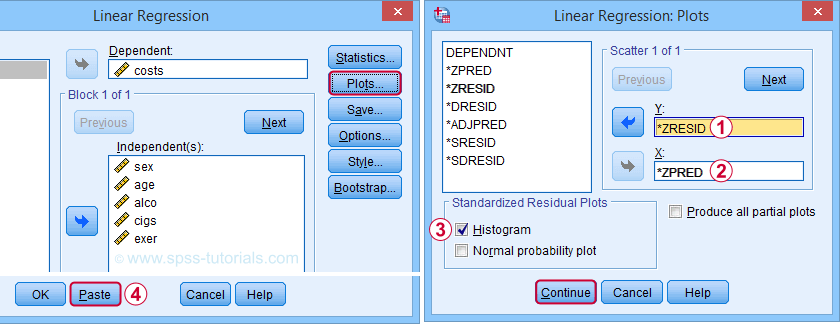
Clicking Paste results in the syntax below. We'll run it and inspect the residual plots shown below.

SPSS Multiple Regression Syntax II

Residual Plots I - Histogram

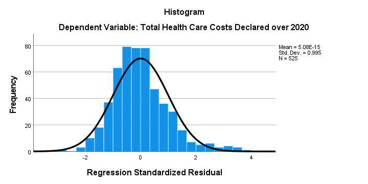
The histogram over our standardized residuals shows

• a tiny bit of positive skewness; the right tail of the distribution is stretched out a bit.
• a tiny bit of positive kurtosis; our distribution is more peaked (or “leptokurtic”) than the normal curve. This is because the bars in the middle are too high and pierce through the normal curve.

In short, we do see some deviations from normality but they're tiny. Most analysts would conclude that the residuals are roughly normally distributed. If you're not convinced, you could add the residuals as a new variable to the data via the SPSS regression dialogs. Next, you could run a Shapiro-Wilk test or a Kolmogorov-Smirnov test on them. However, we don't generally recommend these tests.

Residual Plots II - Scatterplot

The residual scatterplot shown below is often used for checking a) the homoscedasticity and b) the linearity assumptions. If both assumptions hold, this scatterplot shouldn't show any systematic pattern whatsoever. That seems to be the case here.

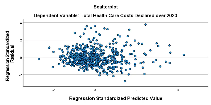
Homoscedasticity implies that the variance of the residuals should be constant. This variance can be estimated from how far the dots in our scatterplot lie apart vertically. Therefore, the height of our scatterplot should neither increase nor decrease as we move from left to right. We don't see any such pattern.

A common check for the linearity assumption is inspecting if the dots in this scatterplot show any kind of curve. That's not the case here so linearity also seems to hold here.On a personal note, however, I find this a very weak approach. An unusual (but much stronger) approach is to fit a variety of non linear regression models for each predictor separately.

Doing so requires very little effort and often reveils non linearity. This can then be added to some linear model in order to improve its predictive accuracy.

Sadly, this “low hanging fruit” is routinely overlooked because analysts usually limit themselves to the poor scatterplot aproach that we just discussed.

APA Reporting Multiple Regression

The APA reporting guidelines propose the table shown below for reporting a standard multiple regression analysis.

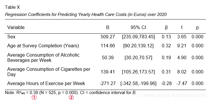
I think it's utter stupidity that the APA table doesn't include the constant for our regression model. I recommend you add it anyway. Furthermore, note that

R-square adjusted is found in the model summary table and
its p-value is the only number you need from the ANOVA table

in the SPSS output. Last, the APA also recommends reporting a combined descriptive statistics and correlations table like we saw here.

Thanks for reading!