Skewness is a number that indicates to what extent
a variable is asymmetrically distributed.

• Positive (Right) Skewness Example
• Negative (Left) Skewness Example
• Population Skewness - Formula and Calculation
• Sample Skewness - Formula and Calculation
• Skewness in SPSS
• Skewness - Implications for Data Analysis

Positive (Right) Skewness Example

A scientist has 1,000 people complete some psychological tests. For test 5, the test scores have skewness = 2.0. A histogram of these scores is shown below.

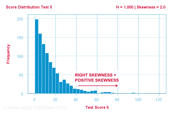
The histogram shows a very asymmetrical frequency distribution. Most people score 20 points or lower but the right tail stretches out to 90 or so. This distribution is right skewed.
If we move to the right along the x-axis, we go from 0 to 20 to 40 points and so on. So towards the right of the graph, the scores become more positive. Therefore, right skewness is positive skewness which means skewness > 0. This first example has skewness = 2.0 as indicated in the right top corner of the graph. The scores are strongly positively skewed.

Negative (Left) Skewness Example

Another variable -the scores on test 2- turn out to have skewness = -1.0. Their histogram is shown below.

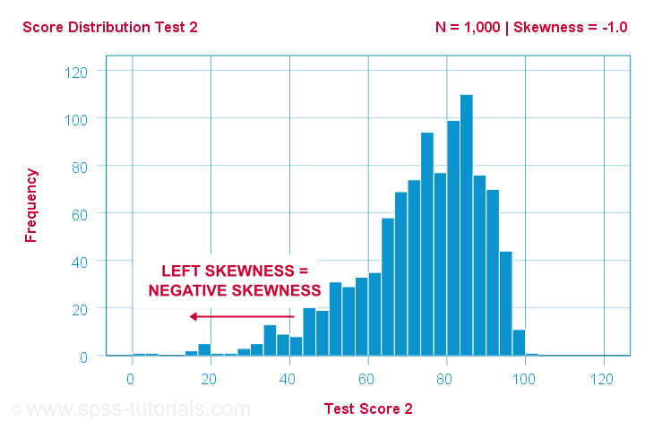
The bulk of scores are between 60 and 100 or so. However, the left tail is stretched out somewhat. So this distribution is left skewed.
Right: to the left, to the left. If we follow the x-axis to the left, we move towards more negative scores. This is why left skewness is negative skewness. And indeed, skewness = -1.0 for these scores. Their distribution is left skewed. However, it is less skewed -or more symmetrical- than our first example which had skewness = 2.0.

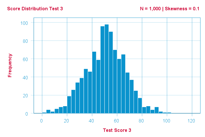
Symmetrical Distribution Implies Zero Skewness

Finally, symmetrical distributions have skewness = 0. The scores on test 3 -having skewness = 0.1- come close.

Now, observed distributions are rarely precisely symmetrical. This is mostly seen for some theoretical sampling distributions. Some examples are

• the (standard) normal distribution;
• the t distribution and
• the binomial distribution if p = 0.5.

These distributions are all exactly symmetrical and thus have skewness = 0.000...

Population Skewness - Formula and Calculation

If you'd like to compute skewnesses for one or more variables, just leave the calculations to some software. But -just for the sake of completeness- I'll list the formulas anyway.
If your data contain your entire population, compute the population skewness as:
$$Population\;skewness = \Sigma\biggl(\frac{X_i - \mu}{\sigma}\biggr)^3\cdot\frac{1}{N}$$
where

• \(X_i\) is each individual score;
• \(\mu\) is the population mean;
• \(\sigma\) is the population standard deviation and
• \(N\) is the population size.

For an example calculation using this formula, see this Googlesheet (shown below).

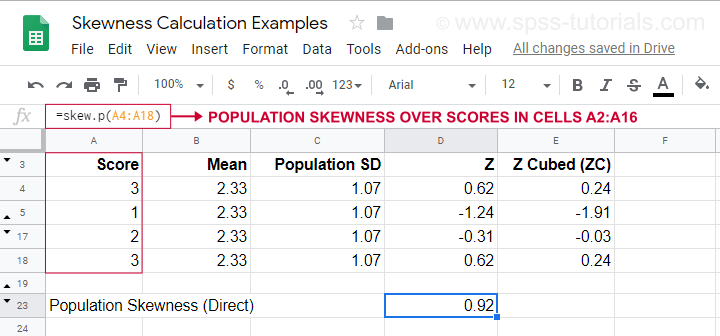
It also shows how to obtain population skewness directly by using =SKEW.P(...) where “.P” means “population”. This confirms the outcome of our manual calculation. Sadly, neither SPSS nor JASP compute population skewness: both are limited to sample skewness.

Sample Skewness - Formula and Calculation

If your data hold a simple random sample from some population, use
$$Sample\;skewness = \frac{N\cdot\Sigma(X_i - \overline{X})^3}{S^3(N - 1)(N - 2)}$$
where

• \(X_i\) is each individual score;
• \(\overline{X}\) is the sample mean;
• \(S\) is the sample-standard-deviation and
• \(N\) is the sample size.

An example calculation is shown in this Googlesheet (shown below).

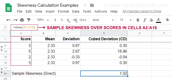
An easier option for obtaining sample skewness is using =SKEW(...). which confirms the outcome of our manual calculation.

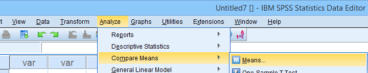
Skewness in SPSS

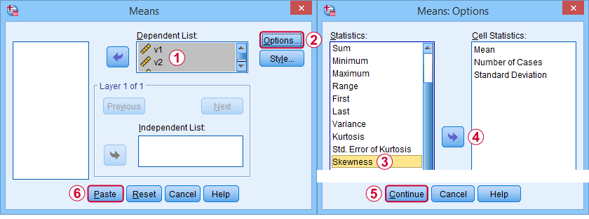
First off, “skewness” in SPSS always refers to sample skewness: it quietly assumes that your data hold a sample rather than an entire population. There's plenty of options for obtaining it. My favorite is via MEANS because the syntax and output are clean and simple. The screenshots below guide you through.

The syntax can be as simple as means v1 to v5
/cells skew. A very complete table -including means, standard deviations, medians and more- is run from means v1 to v5
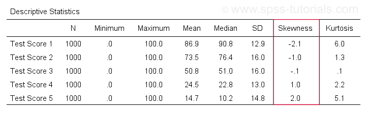
/cells count min max mean median stddev skew kurt. The result is shown below.

Skewness - Implications for Data Analysis

Many analyses -ANOVA, t-tests, regression and others- require the normality assumption: variables should be normally distributed in the population. The normal distribution has skewness = 0. So observing substantial skewness in some sample data suggests that the normality assumption is violated.
Such violations of normality are no problem for large sample sizes -say N > 20 or 25 or so. In this case, most tests are robust against such violations. This is due to the central limit theorem. In short, for large sample sizes, skewness is
no real problem for statistical tests. However, skewness is often associated with large standard deviations. These may result in large standard errors and low statistical power. Like so, substantial skewness may decrease the chance of rejecting some null hypothesis in order to demonstrate some effect. In this case, a nonparametric test may be a wiser choice as it may have more power. Violations of normality do pose a real threat
for small sample sizes of -say- N < 20 or so. With small sample sizes, many tests are not robust against a violation of the normality assumption. The solution -once again- is using a nonparametric test because these don't require normality.
Last but not least, there isn't any statistical test for examining if population skewness = 0. An indirect way for testing this is a normality test such as

• the Kolmogorov-Smirnov normality test and
• the Shapiro-Wilk normality test.

However, when normality is really needed -with small sample sizes- such tests have low power: they may not reach statistical significance even when departures from normality are severe. Like so, they mainly provide you with a false sense of security.

And that's about it, I guess. If you've any remarks -either positive or negative- please throw in a comment below. We do love a bit of discussion.

Thanks for reading!