For reading up on some basics, see ANOVA - What Is It?.

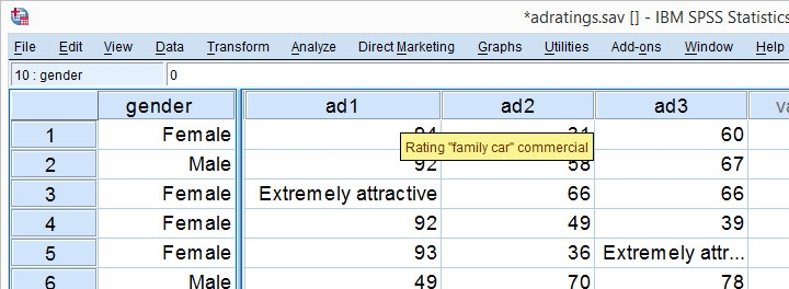
A car brand had 18 respondents rate 3 different car ads on attractiveness. The resulting data -part of which are shown above- are in adratings.sav. Some background variables were measured as well, including the respondent’s gender. The question we'll try to answer is: are the 3 ads rated equally attractive and does gender play any role here? Since we'll compare the means of 3(+) variables measured on the same respondents, we'll run a repeated measures ANOVA on our data. We'll first overview a simple but solid approach for the entire process. We'll then explain the what and why of each of these steps as we'll carry out the analysis step-by-step.

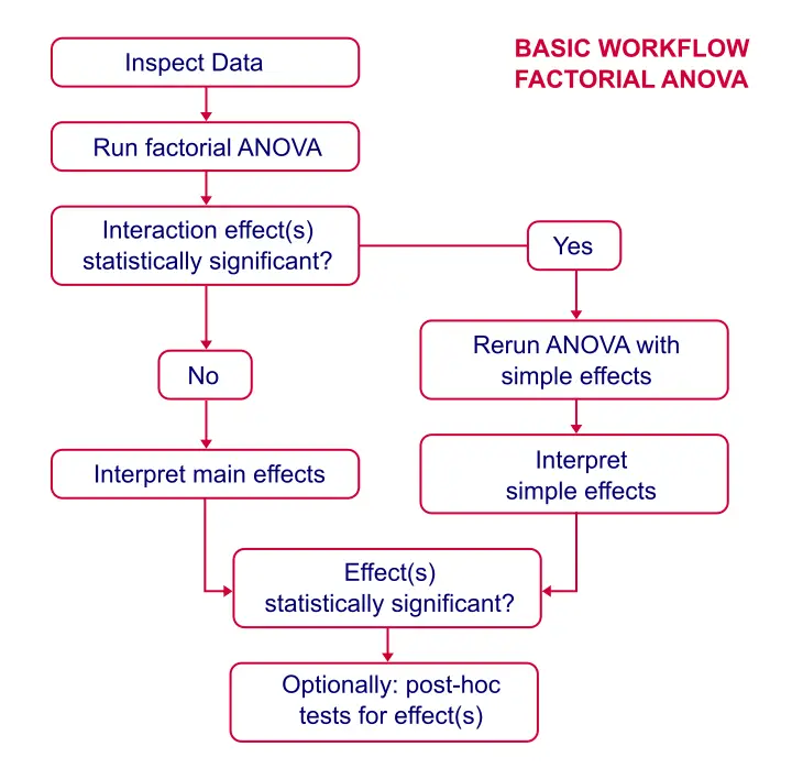
Factorial ANOVA - Basic Workflow

Data Inspection

First, we're not going to analyze any variables if we don't have a clue what's in them. The very least we'll do is inspect some histograms for outliers, missing values or weird patterns. For gender, a bar chart would be more appropriate but the histogram will do.

SPSS Basic Histogram Syntax

You can now verify for yourself that all distributions look plausible and there's no missing values or other issues with these variables.

Assumptions for Repeated Measures ANOVA

1. Independent and identically distributed variables (“independent observations”).
2. Normality: the test variables follow a multivariate normal distribution in the population.
3. Sphericity: the variances of all difference scores among the test variables must be equal in the population.^{1, 2, 3}

First, since each case (row of data cells) in SPSS holds a different person, the observations are probably independent.
Regarding the normality assumption, our previous histograms showed some skewness but nothing too alarming.
Last, Mauchly’s test for the sphericity assumption will be included in the output so we'll see if that holds in a minute.

Running Repeated Measures ANOVA in SPSS

We'll first run a very basic analysis by following the screenshots below. The initial results will then suggest how to nicely fine tune our analysis in a second run.

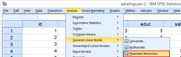
Repeated Measures may be absent from your menu if you don't have the SPSS option “Advanced statistics” installed. You can verify this by running show license.

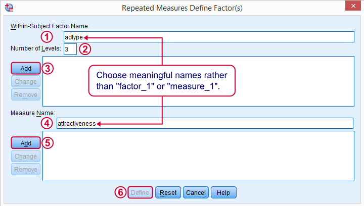
The within-subjects factor is whatever distinguishes the three variables we'll compare. We recommend you choose a meaningful name for it.

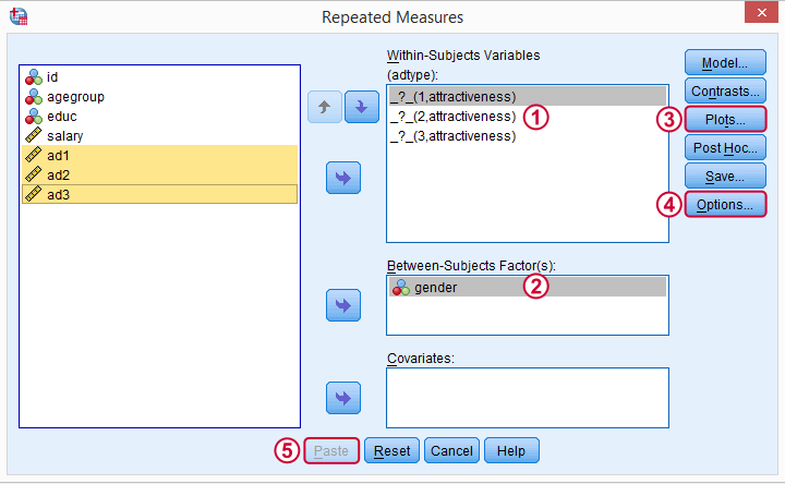
Select and move the three adratings variables in one go to the within-subjects variables box. Move gender into the between-subjects factor box.

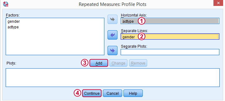
These profile plots will nicely visualize our 6 means (3 ads for 2 genders) in a multiple line chart.

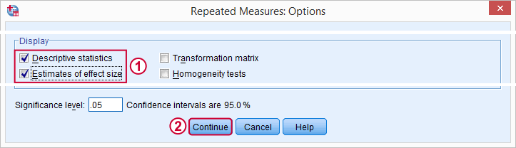
For now, we'll only tick Descriptive Statistics and Estimates of Effect Size in the Options subdialog. Clicking Paste in the main dialog results in the syntax below.

SPSS Basic Repeated Measures ANOVA Syntax

Output - Select and Reorder

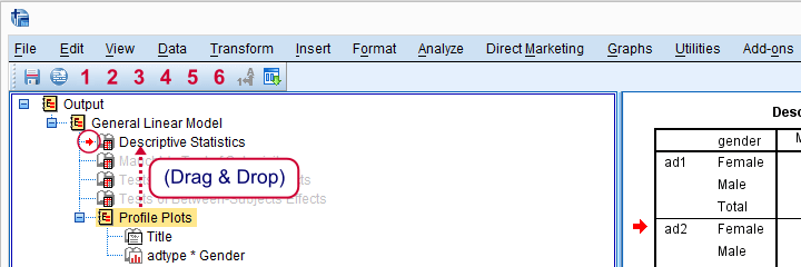
Since we're not going to inspect all of our output, we'll first delete some items as shown below.

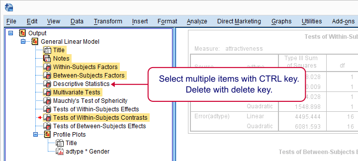
Next, we'll move our profile plots up by dragging and dropping it right underneath the descriptive statistics table.

Output - Means Plot and Descriptives

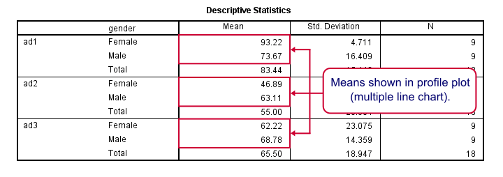
At the very core of our output, we just have 6 means: 3 ads for men and women separately. Both men and women rate adtype 1 (“family car”, as seen in the variable labels) most attractive. Adtype 2 (“youngster car”) is rated worst and adtype 3 is in between.Technical note: these means may differ from DESCRIPTIVES output because the repeated measures procedure excludes all cases with one or more missing values from the entire procedure.

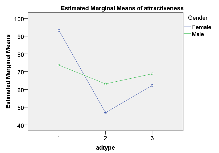
These means are nicely visualized in our profile plot.The “estimated marginal means” are equal to the observed means for the saturated model (all possible effects included). By default, SPSS always tests the saturated model for any factorial ANOVA. Now, what's really important is that the lines are far from parallel. This suggests an interaction effect: the effect of adtype is different for men and women.
Roughly, the line is almost horizontal for men: the three ads are rated quite similarly. For women, however, there's a huge difference between ad1 and ad2.
Keep in mind, however, that this is just a sample. Are the differences we see large enough for concluding anything about the entire population from which our sample was drawn? The answer is a clear “yes!” as we'll see in a minute.

Output - Mauchly’s Test

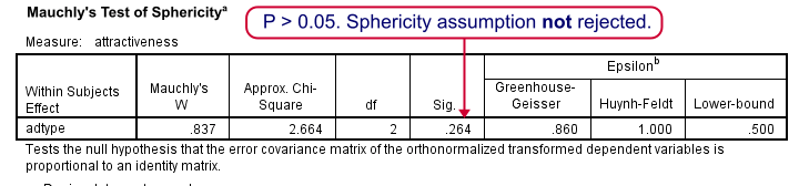
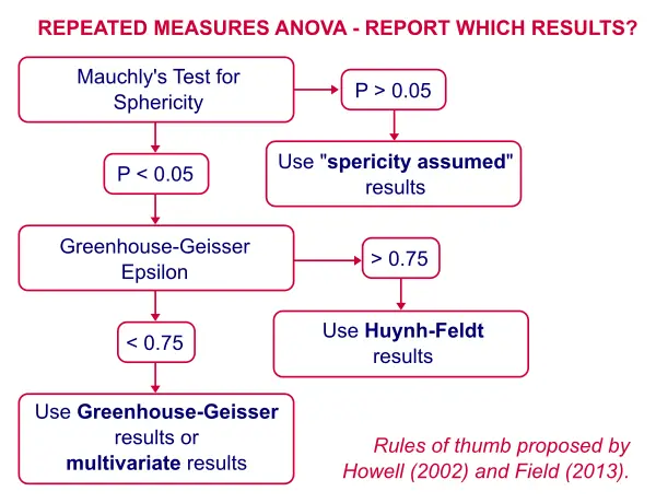
As we mentioned under assumptions, repeated measures ANOVA requires sphericity and Mauchly’s test evaluates if this holds. The p-value (denoted by “Sig.”) is 0.264. We usually state that sphericity is met if p > 0.05, so the sphericity assumption is met by our data. We don't need any correction such as Greenhouse-Geisser of Huynh-Feldt. The flowchart below suggests which results to report if sphericity does (not) hold.

Output - Within-Subjects Effects

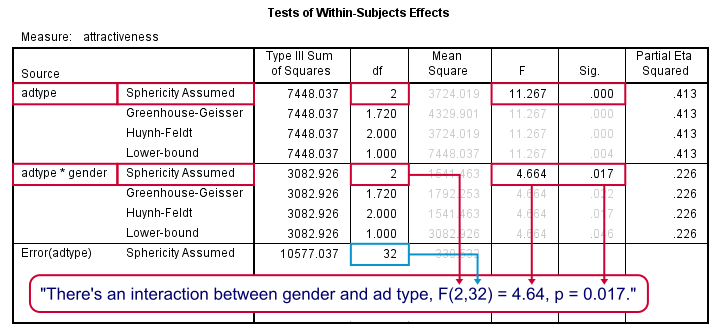
First, the interaction effect between gender and adtype has a p-value (“Sig.”) of 0.017. If p < 0.05, we usually label an effect “statistically significant” so we have an interaction effect indeed as suggested by our profile plot.
This plot shows that the effects for adtype are clearly different for men and women. So we should test the effects of adtype for male and female respondents separately. These are called simple effects as shown in our flowchart.
There is a strong main effect for adtype: F(2,32) = 11.27, p = 0.000 too. But as suggested by our flowchart, we'll ignore it. The main effect lumps together men and women, which is justifiable only if these show similar effects for adtype. That is: if the lines in our profile plot would run roughly parallel but that's not the case here.
In other words, there's no such thing as the effect of adtype as a main effect suggests. The separate effects of adtype for men and women would be obscured by taking them together so we'll analyze them separately (simple effects) instead.

Repeated Measures ANOVA - Simple Effects

There's no such thing as “simple effects” in SPSS’ menu. However, we can easily analyze male and female respondents separately with SPLIT FILE by running the syntax below.

Repeated Measures ANOVA - Second Run

The SPLIT FILE we just allows us to analyze simple effects: repeated measures ANOVA output for men and women separately. We can either rerun the analysis from the main menu or use the dialog recall button as a handy shortcut.

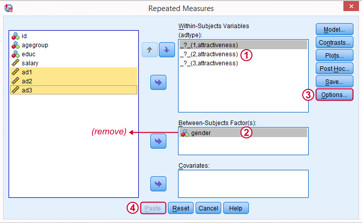
We remove gender from the between-subjects factor box. Because the analysis is run for men and women separately, gender will be a constant in both groups.

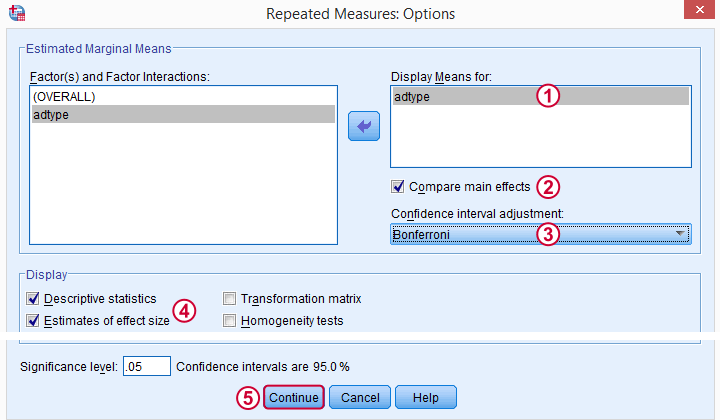
As suggested by our flowchart, we'll now add some post hoc tests. Post hoc tests for within-subjects factors (adtype in our case) are well hidden behind the Options rather than the Post Hoc button. The latter only allows post hoc tests for between-subjects effects, which we no longer have.

Repeated Measures ANOVA - Simple Effects Syntax

Simple Effects - Output

We interpret most output as previously discussed. Note that adtype has an effect for female respondents: F(2,16) = 11.68, p = 0.001. The precise meaning of this is that if all three population mean ratings would be equal, we would have a 0.001 (or 0.1%) chance of finding the mean differences we observe in our sample.
For males, this effect is not statistically significant: F(2,16) = 1.08, p = .362: if the 3 population means are really equal, we have a 36% chance of finding our sample differences; what we see in our sample does not negate our null hypothesis.

Output - Post Hoc Tests

Right, we just concluded that adtype is related to rating for female but not male respondents. We'll therefore interpret the post hoc results for female respondents only and ignore those for male respondents.
But why run post hoc tests in the first place? Well, we concluded that the null hypothesis of all population mean rating equal is not tenable. However, with 3 or more means, we don't know exactly which means are different. A post hoc (Latin for “after that”) test -as suggested by our flowchart- will tell us just that.

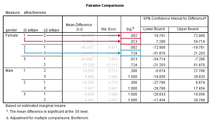
With 3 means, we've 3 comparisons and each of them is listed twice in this table; 1 versus 3 is obviously the same as 3 versus 1. We quickly see that ad1 differs from ad2 and ad3. The difference between ad2 and ad3, however, is not statistically significant. Unfortunately, SPSS doesn't provide the t-values and degrees of freedom needed for reporting these results.
An alternative way to obtain these is running paired samples t-tests on all pairs of variables. The Bonferroni correction means that we'll multiply all p-values by the number of tests we're running (3 in this case). Doing so is left as an exercise to the reader.

Thanks for reading!

References

1. Field, A. (2013). Discovering Statistics with IBM SPSS Newbury Park, CA: Sage.
2. Howell, D.C. (2002). Statistical Methods for Psychology (5th ed.). Pacific Grove CA: Duxbury.
3. Wijnen, K., Janssens, W., De Pelsmacker, P. & Van Kenhove, P. (2002). Marktonderzoek met SPSS: statistische verwerking en interpretatie [Market Research with SPSS: statistical processing and interpretation]. Leuven: Garant Uitgevers.